Open Stacked Rapid Sand Filter Design

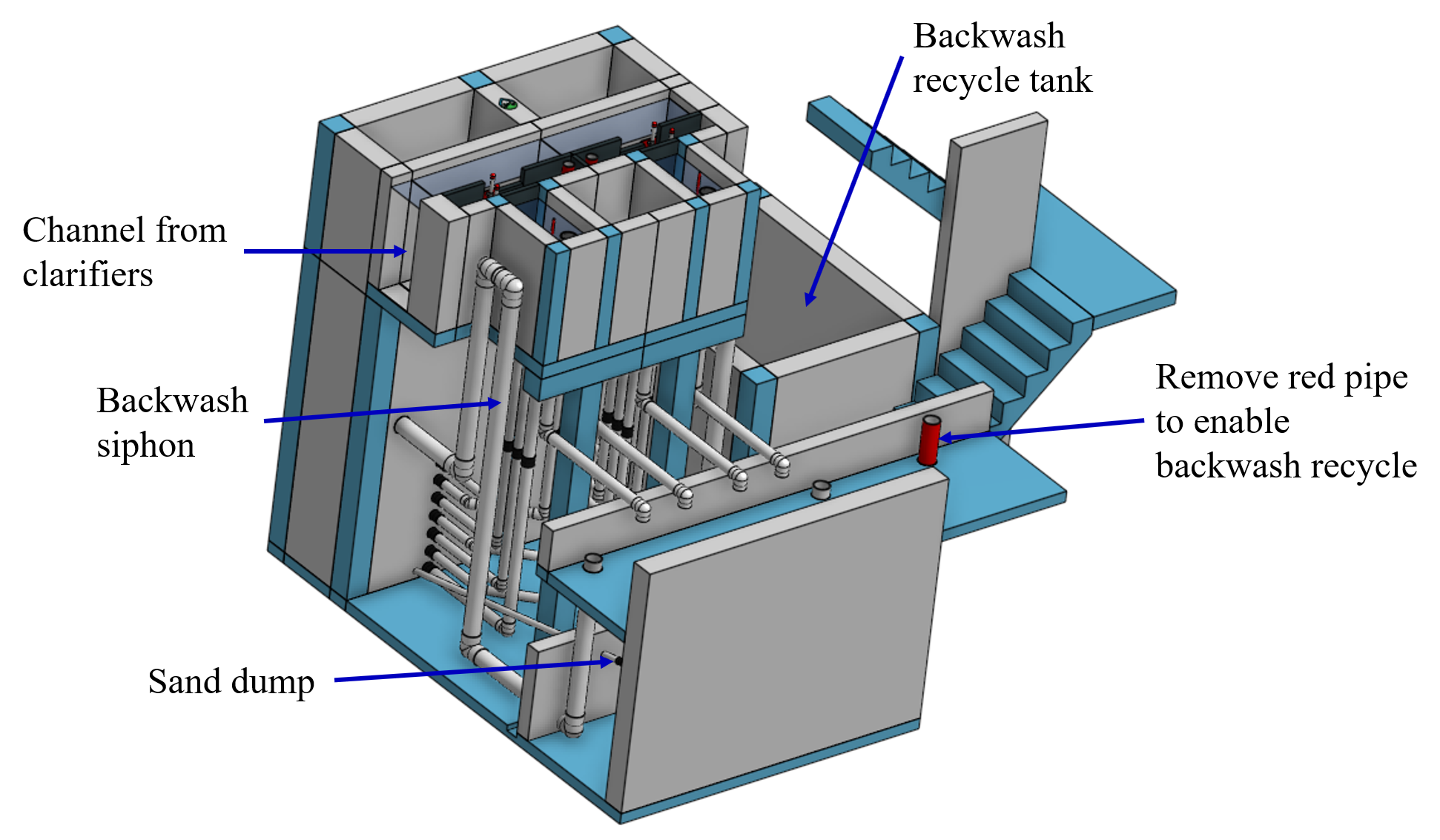
Fig. 204 The open stacked rapid sand filters include advanced hydraulic controls to ensure stable operation during both filtration and backwash modes.

Nomenclature

B - branch

P - port (or orifice)

T - trunk

Introduction

The hydraulic design of both the enclosed and open stacked rapid sand filter is complicated by the number of parallel flows, the manifolds in series, and the need to handle both backwash and filter modes. The design requires careful attention to weir hydraulics to achieve the target backwash flows when the plant is operating at less than full capacity. The siphon system has a tight design constraint to ensure that the siphon doesn’t trigger prematurely.

Filter Inlet Channel with Rectangular Weir Flow Distribution

In plants with flow rates large enough to use open stacked rapid sand filters the settled water is delivered to those filters through an open channel. The water exits the channel by flowing across a rectangular weir (see Fig. 205). As is the case in a manifold pipe the water in the channel is decelerating and thus the piezometric head is increasing in the direction of flow. This increase in piezometric head is equivalent to the increase in the depth of water in the channel. This increase in water depth results in more water flowing across the final weir exiting the channel.

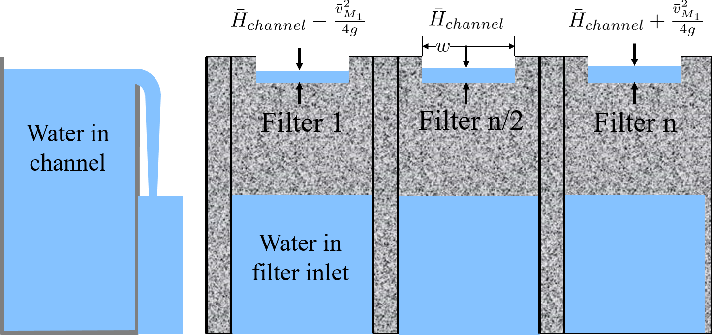
Fig. 205 The filter inlet channel distributes flow to all of the filters. The water in the channel flows across sharp crested weirs into the filter inlet boxes. The velocity in the channel decreases in the direction of flow and thus the kinetic energy of the flow is converted into height. That added height results in greater flow into downstream filter inlet boxes.

The flow across the weirs into the filter inlet boxes is complicated by several factors. First, there must be a vena contracta as the flow changes direction to flow across the weir and thus the \(90^{\circ}\) vena contracta coefficient should enter the equations. Second, the weirs as they are fabricated are neither sharp nor broad and thus it isn’t clear which equations are best suited. Sharp crested weirs are known to have a reduced depth of flow above the weir due to the acceleration of water approaching the weir and this effect is normally ignored and then thrown into the weir coefficient. Given that our weirs do not have a rounded upstream edge required by broad crested weirs we will use the sharp crested weir equation.

Side Exit Sharp Crested Weir

(274)\[ Q = \Pi_{vc}\frac{2}{3} \sqrt{2g} w \left(H_{channel}\right)^\frac{3}{2}\]

where \(H_{channel}\) is the height of the water in the channel above the top of the weir. (see equation 10.30 in Fundamentals of Fluid Mechanics, Fifth Edition by Munson, Young, and Okiishi)

Inlet Channel Design for Equal Filter Flow

We will simplify this manifold problem by assuming that the average water height in the channel above the weirs corresponds to the average flow across the weirs and that the upstream depth is decreased by 1/2 of the channel velocity head and the downstream depth is increased by 1/2 the channel velocity head.

The ratio of flows from the first filter and the last filter in the channel is given by

(275)\[\Pi_{Q_{weir}} = \frac{Q_{Filter_1}}{Q_{Filter_n}} = \frac{\Pi_{vc}\frac{2}{3} \sqrt{2g} w \left(\bar H_{channel} - \frac{\bar v_{M_1}^2}{4g}\right)^\frac{3}{2}}{\Pi_{vc}\frac{2}{3} \sqrt{2g} w \left(\bar H_{channel} + \frac{\bar v_{M_1}^2}{4g}\right)^\frac{3}{2}}\]

where \(\bar H_{channel}\) is the average height of water in the channel relative to the top of the weir. Equation (275) simplifies to

(276)\[\Pi_{Q_{weir}} = \frac{ \left(\bar H_{channel} - \frac{\bar v_{M_1}^2}{4g}\right)^\frac{3}{2}}{\left(\bar H_{channel} + \frac{\bar v_{M_1}^2}{4g}\right)^\frac{3}{2}}\]

The slower the velocity in the channel the more uniform the flow distribution will be between the filters.

Solve for the maximum velocity in the channel given the average depth of water above the weirs and the required flow distribution.

(277)\[ \bar H_{channel}\Pi_{Q_{weir}}^\frac{2}{3} + \frac{\bar v_{M_1}^2}{4g}\Pi_{Q_{weir}}^\frac{2}{3}= { \bar H_{channel} - \frac{\bar v_{M_1}^2}{4g}}\]

Now we can solve for maximum manifold channel velocity.

(278)\[\bar v_{M_1} = 2\sqrt{g\bar H_{channel}\frac{\left(1-\Pi_{Q_{weir}}^\frac{2}{3}\right)}{\left(\Pi_{Q_{weir}}^\frac{2}{3} + 1\right)}}\]

The channel depth of water above the weir, \(\bar H_{channel}\), and the flow uniformity target set the maximum velocity in the manifold channel (see Fig. 206).

Generate the following plot

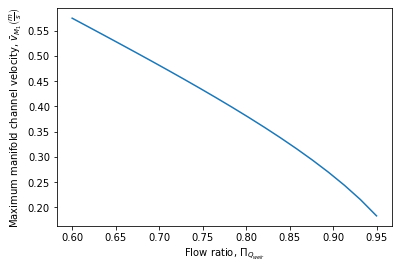
Fig. 206 The maximum velocity in the filter inlet channel decreases as the target flow ratio, \(\Pi_{Q_{weir}}\), approaches 1. This graph was created assuming \(\bar H_{channel}\) of 5 cm.

Backwash Weir Slot Design

The goal of the backwash weir slot is to provide close to the design flow rate to a filter while it is in backwash mode. To accomplish this the wide gate weir is opened and the weir slot controls the flow of water into the inlet box. During backwash the water level in the inlet box is much lower and thus the backwash weir slot can extend deep into the box. The design constraint for this slot is that it must deliver the design flow when the water level in the inlet channel is at the design flow height and it must deliver at least 80% of the design flow when there is no flow going to any of the other filters. The difference in water level between the two cases is \(H_{channel}\) because this is the height of water flowing over the wide weir at the design flow rate. The height of the slot, \(H_{slot}\), is measured relative to the design flow water level in the inlet channel.

This design will result in more water available for backwash than is absolutely needed and if it turns out that too much water is directed to this filter than the bottom of the slot can be elevated by adding a few stop logs.

The equation is based on the sharp crested weir (Equation (274)). The head loss through the gate weir should be subtracted from both the top and bottom terms

(279)\[\Pi_{Q_{BW}} = \frac{Q_{BW_{min}}}{Q_{BW_{max}}} = \frac{\Pi_{vc}\frac{2}{3} \sqrt{2g} w \left(H_{slot} - H_{channel} - HL_{Gate}\right)^\frac{3}{2}}{\Pi_{vc}\frac{2}{3} \sqrt{2g} w \left(H_{slot}- HL_{Gate}\right)^\frac{3}{2}}\]

Simplify and solve for \(H_{slot}\).

(280)\[ H_{slot} = \frac{H_{channel}}{1-\Pi_{Q_{BW}}^\frac{2}{3}} + HL_{Gate}\]

There are two possible constraints on the trunk size. Either the trunk size is dictated by backwash flow distribution requirements or the trunk size is dictated by the need to have uniform flow distribution between filter layers and hence to have exactly twice the flow rate through the inner inlets.

There are 4 levels of flow distribution in StaRS filters. The direction of the design (top-down or bottom-up) is determined by the fact that when there is head loss in series that all of the head loss helps to achieve flow distribution. Thus the head loss through the orifices will be a required part of the design of the branches and that head loss will be an input for the trunk design. Thus we need to start at the bottom and work up.

• between orifices (branchPortQ_pi): made less important by the winged design that allows correcting flow in the winged space before the water enters the sand bed. This flow distribution does not benefit from the head loss through the sand. Suggest using a value of 0.8 for this constraint because of the balancing provided by the wings. The flow distribution constraint only provides a ratio of the port and branch velocities. The constraint for the maximum velocity allowable is either set by head loss or by the strength of the branch to span its length and not bend to much at the initiation of backwash. Either of those constraints can be converted into a maximum velocity for the inner branches and that will be used as an input to the design.

  • The velocity constraint will determine the maximum length of a branch given its diameter.

  • Use Equation (43) combined with the maximum branch velocity constraint to calculate the port velocity. Calculate the required branch diameter given the length (or vice versa).

  • The orifice diameter will be selected based on constructability and not being too small to risk clogging (between 4 and 10 mm)

  • Calculate the orifice spacing for the inner branches based on mass conservation and the maximum port velocity.

  • Calculate the maximum length of the branches given mass conservation and the maximum branch velocity.

• between branches (trunkPortQ_pi): aided considerably by the head loss through the sand and is helped by the head loss though the orifices. Suggest using a value of 0.9 for this constraint. This constraint will be combined with a maximum permissible head loss during backwash to determine the required diameter of the trunk lines and will be combined with the equal trunk head loss constraint to obtain the diameter of the orifices.

  • Use Equation (42) to solve for the maximum trunk velocity.

  • Use the fact that the head loss is the same for outer and inner inlets to determine the \(K_{e_{outerOrifices}}\).

• between sand layers: easily obtained by simply requiring that inlet head losses be identical in the 4 inlets under conditions of the target flow and accounting for the fact that the inner inlets have double the flow of the outer inlets.

• between filters: will be handled by design of the weirs into the filter inlet boxes

The clean bed sand head loss and including the head loss right at the point where the water enters the sand helps with the flow distribution between branches and between orifices. We are not currently including the benefit of the high velocity at the point where the water enters the sand.

Design Steps

Inner Trunk

The diameter of the trunk lines is set by the filtration flow distribution between ports in the inner trunks and the maximum acceptable inlet head loss during backwash. The backwash head loss constraint is directly connected to the head loss during filtration because the velocity in the backwash trunk changes by a factor of the number of filter layers. The backwash inlet head loss sets the required depth of the open filter box and so is an important constraint for O-StaRS. Both the inner and outer inlet head loss during filtration is \(\frac{1}{N_{layers}^2}\) times the backwash inlet head loss because the head loss is proportional to the flow ratio squared and because we will set the inlet head losses to be identical during filtration.

The equation for flow distribution between branches with additional head loss in series is (42).

(281)\[ \frac{\bar v_{T_{innerMax}}^2}{2g}= \left(h_{e_{B_{inner}}} + h_{e_{P_{inner}}} + h_{l_{sand}} \right)\Pi_{\Psi_B}\]

The head loss through the inner ports or orifices required to achieve reasonable flow distribution into the winged area of the inlet branches can be expressed in the minor loss equation form. The flow distribution constraint is given by Equation (43).

(282)\[h_{e_{P_{inner}}} = \frac{\bar v_{P_{inner}}^2}{2g} = \frac{\bar v_{B_{inner}}^2}{2g}\frac{1}{\Pi_{\Psi_P}}\]

where the port velocity \(\bar v_{P_{inner}}\) is the contracted velocity out of the orifice.

The branch entrance loss is given by

(283)\[h_{e_{B_{inner}}} = K_{e_B}\frac{\bar v_{B_{innerMax}}^2}{2g}\]

The minor loss associated with entering the branch is given by Equation (283)). The \(h_{l_{series}}\) is the sum of the orifice head loss (see Equation (282)) and the head loss through the sand. Making those substitutions into Equation (281) we obtain

(284)\[ \bar v_{T_{innerMax}}^2 = \Pi_{\Psi_B}\left[\bar v_{B_{innerMax}}^2\left(K_{e_B} + \frac{1}{\Pi_{\Psi_P}}\right) + 2gh_{l_{sand}} \right]\]

This is a constraint on the maximum branch velocity assuming that the port velocity is set to achieve flow distribution to the wings within a branch (rather than setting the port velocity to achieve flow distribution between branches).

This shows that the trunk velocity is limited by the branch velocity even without applying the head loss constraint. However, even if the branch velocity approaches zero, the trunk velocity can still be quite high because of the balancing effect of the sand head loss. This constraint ends up not being useful because flow division between branches is not a critical constraint.

The head loss constraint is

(285)\[h_{e_{outerInlet_{Bw}}} = N_{layer}^2 h_{e_{innerInlet}} = N_{layer}^2 \left(h_{e_{T_{inner}}} + h_{e_{B_{inner}}} + h_{e_{P_{inner}}} \right)\]

The trunk entrance and elbow losses are given by

(286)\[h_{e_{T_{inner}}} = K_{e_T}\frac{\bar v_{T_{innerMax}}^2}{2g}\]

Substitute with minor loss relationships.

(287)\[2gh_{e_{outerInlet_{Bw}}} = N_{layer}^2 \left(K_{e_T}\bar v_{T_{innerMax}}^2 + K_{e_B}\bar v_{B_{innerMax}}^2 + \bar v_{B_{innerMax}}^2\frac{1}{\Pi_{\Psi_P}} \right)\]

Solve for \(\bar v_{T_{innerMax}}\).

(288)\[\bar v_{T_{innerMax}} = \sqrt{\frac{2gh_{e_{outerInlet_{Bw}}}}{K_{e_T} N_{layer}^2} -\frac{\bar v_{B_{innerMax}}^2}{K_{e_T}}\left(K_{e_B} + \frac{1}{\Pi_{\Psi_P}} \right)}\]

The head loss constraint reveals that we can achieve the highest trunk velocity by setting the branch velocity to zero! This is because the branch head loss is not needed to achieve flow distribution between branches. Thus we will design the branches to have low velocities to increase the flow that can be achieved with a given size trunk. First define a dimensionless ratio of branch to trunk kinetic energy that will be used as a user specified constraint to allow the exploration of the tradeoff.

(289)\[\bar v_{B_{innerMax}}^2 = \Pi_{BT} \bar v_{T_{innerMax}}^2\]

Use Equation (289) to eliminate \(\bar v_{B_{innerMax}}\) in Equation (287).

(290)\[2gh_{e_{outerInlet_{Bw}}} = N_{layer}^2 \left(K_{e_T}\bar v_{T_{innerMax}}^2 + K_{e_B}\Pi_{BT} \bar v_{T_{innerMax}}^2 + \Pi_{BT} \bar v_{T_{innerMax}}^2\frac{1}{\Pi_{\Psi_P}} \right)\]

solve for \(\bar v_{T_{innerMax}}\).

(291)\[\bar v_{T_{innerMax}} = \sqrt{\frac{2gh_{e_{outerInlet_{Bw}}}}{N_{layer}^2 \left[K_{e_T} + \Pi_{BT}\left(K_{e_B} + \frac{1}{\Pi_{\Psi_P}} \right)\right]}}\]

Inner branch

Use Equation (289) to solve for the maximum branch velocity given the results from Equation (291).

Given the constraint of maximum branch velocity use the relationship between port velocity and branch velocity given by Equation (43) to solve for the port velocity.

(292)\[\bar v_{P_{innerMax}} = \bar v_{B_{innerMax}}\sqrt{\frac{1}{\Pi_{\Psi_P}}}\]

The orifice diameter will be constrained by the wing fabrication. Apply conservation of mass to obtain the port velocity to filter velocity ratio. Each port serves an area equal to the branch spacing times the port spacing.

(293)\[\frac{\bar v_{P_{innerMax}}}{2 v_{Fi}} = \frac{B_{branch} B_{orifice_{inner}}}{\Pi_{vc}\frac{\pi}{4} D_{orifice}^2}\]

where the factor of 2 is because the inner trunks serve two layers of sand. Combine equations (292) and (293) and solve for the center to center spacing of the orifices.

(294)\[B_{orifice_{inner}} = \frac{\bar v_{B_{innerMax}}\Pi_{vc}\pi D_{orifice}^2}{8 v_{Fi}B_{branch}}\sqrt{\frac{1}{\Pi_{\Psi_P}}}\]

We will assume that the user sets the target branch diameter as an input. The maximum length of a branch is set by mass conservation and the flow required to serve the filter area corresponding to the length of the branch.

(295)\[2 v_{Fi} L_{branch_{max}} B_{branch} = \bar v_{B_{innerMax}} A_{pipe}\]

Solve for \(L_{branch_{max}}\).

(296)\[ L_{branch_{max}} = \frac{\bar v_{B_{innerMax}} A_{pipe}}{2 v_{Fi} B_{branch}}\]

Solve for the minimum pipe ID.

(297)\[ D_{branch_{min}}= \sqrt\frac{8 v_{Fi} B_{branch} L_{branch}}{\pi \bar v_{B_{innerMax}}}\]

At this stage in the design process we have set the flow rate through the filter, the trunk and branch diameters (except for the backwash branches), the length of the branches, and the orifice spacing on the inner inlets.

Outer branch

The outer trunk branch orifices must be designed so that the head loss during filtration is identical between inner and outer inlets. This will result spacing between the outer branch orifices that is more than double that of the inner branch orifices. The derivation is similar to that used to obtain Equation (294). Equate the head loss in the inner and outer inlets during filtration. We will use the maximum velocity in the inner trunks as our reference velocity. Note that the results would be the same if we used the actual velocity in the inner trunks because the velocity will drop out of the equation in the end. First the head loss from the inlet box to the orifices in the inner inlets is given by

(298)\[2gh_{e_{innerInlet}} = \left(K_{e_T}\bar v_{T_{inner}}^2 + K_{e_B}\bar v_{B_{inner}}^2 + \bar v_{B_{inner}}^2\frac{1}{\Pi_{\Psi_P}} \right)\]

Substitute Equation (289) to eliminate \(\bar v_{B_{inner}}\).

(299)\[2gh_{e_{innerInlet}} = \left[K_{e_T} + \Pi_{BT}\left( K_{e_B} + \frac{1}{\Pi_{\Psi_P}}\right) \right]\bar v_{T_{inner}}^2\]

The orifices for the outer inlets are not constrained by the flow distribution to the ports. Thus the factor \(\frac{1}{\Pi_{\Psi_P}}\) does not apply. The unknown that we are solving for is port velocity which we will obtain from the ratio between port and branch kinetic energy.

(300)\[\bar v_{P_{outer}}^2 = \Pi_{PB_{outer}} \bar v_{B_{outer}}^2\]

The head loss in the outer inlet is given by

(301)\[2gh_{e_{outerInlet}} = \left(K_{e_T} + K_{e_B}\Pi_{BT} + \Pi_{BT} \Pi_{PB_{outer}} \right)\frac{1}{4}\bar v_{T_{inner}}^2\]

where the factor of 4 difference is because the velocity in the outer inlets is half the inner inlets because each inner inlet serves 2 filter layers. Now set the inner and outer head loss to be equal.

(302)\[\left(K_{e_T} + K_{e_B}\Pi_{BT} + \Pi_{BT} \Pi_{PB_{outer}} \right)\frac{1}{4}\bar v_{T_{inner}}^2 = \left(K_{e_T} + K_{e_B}\Pi_{BT} + \Pi_{BT} \frac{1}{\Pi_{\Psi_P}} \right)\bar v_{T_{inner}}^2\]

Simplify and solve for the unknown, \(\Pi_{PB}\).

(303)\[\Pi_{PB_{outer}}= \left(3\frac{K_{e_T}}{\Pi_{BT}} + 3K_{e_B} + 4\frac{1}{\Pi_{\Psi_P}} \right)\]

Apply conservation of mass to obtain the port velocity to filter velocity ratio. Each port serves an area equal to the branch spacing times the port spacing.

(304)\[\frac{\bar v_{P_{outer}}}{v_{Fi}} = \frac{B_{branch} B_{orifice_{outer}}}{\Pi_{vc}\frac{\pi}{4} D_{orifice}^2}\]

We need an equation for \(\bar v_{P_{outer}}\) as a function of \(\bar v_{T_{inner}}\).

(305)\[\frac{1}{4} \bar v_{T_{innerMax}}^2 = \bar v_{T_{outerMax}}^2\]

(306)\[\bar v_{B_{outerMax}}^2 = \Pi_{BT} \bar v_{T_{outerMax}}^2\]

(307)\[\bar v_{P_{outerMax}}^2 = \Pi_{PB_{outer}} \bar v_{B_{outerMax}}^2\]

Combine the previous 3 equations to obtain

(308)\[\bar v_{P_{outerMax}} = \frac{\bar v_{T_{innerMax}}}{2} \sqrt{\Pi_{PB_{outer}} \Pi_{BT}}\]

The orifice spacing should be designed based on the maximum inner trunk velocity rather than the actual inner trunk velocity so that the branches have the same design for all filters. Otherwise the orifice spacing would be different for every design and that would only make fabrication needlessly confusing.

Substitute Equation (308) into Equation (304) and solve for \(B_{orifice_{outer}}\).

(309)\[B_{orifice_{outer}} = \frac{\bar v_{T_{innerMax}} \Pi_{vc} \pi D_{orifice}^2 \sqrt{\Pi_{PB_{outer}} \Pi_{BT}} }{8 v_{Fi} B_{branch}}\]

The backwash branches have an additional constraint. Those branches have two additional challenges. First, during backwash the sand doesn’t provide head loss to help equalize flow. Second, the velocity is \(N_{layer}\) faster than during filtration. We will ensure that the flow is reasonably distributed by applying the flow distribution requirement without any additional head loss in series. We will use the orifice spacing that is used for the outer inlets.

High Flow Design

The flow rate through the filter is severely limited if we keep the constraint that the head loss in the backwash inlet and in the inner inlets be the same. We can uncouple the head loss during the two states by having a removable orifice that can be added to the backwash inlet pipe during filtration.

Design inputs discussion

We could start with a filter width (required by the control system) or a structural constraint given a nominal diameter of the branches. If we start with these two constraints, overall filter width and ND of the branches the branch velocity can be calculated from mass conservation. The complication is that the trunks create an inactive zone in the filter whose width will be a function of the diameter of the trunk and an iterative solution may be required.

A design goal might be to use identical branches for filters of different sizes. That would require setting the branch length as an input rather than the filter width. This might be reasonable and in any case the maximum branch length is a function of the branch ND.

Design steps:

• find the maximum velocity in the outlet branches to get flow distribution through the slots using the filter clean bed head loss. assume branch length and branch ND (or an array of paired options)

• calculate branch velocity from mass conservation

• calculate max trunk velocity using Equation (288)

• size the trunk, then calculate number of filters, flow per filter, filter width, filter length

What are the failure modes as we increase the velocity in the trunk?

• port velocities may have to increase if the sand head loss isn’t sufficient to ensure flow distribution between branches. Higher port velocities could erode the sand under the wing.

• increased inlet head loss requires a deeper filter and deeper inlet and outlet control boxes. It would seem reasonable to limit this head loss to something less than 20 cm given that the dirty bed head loss for the filter is approximately 80 cm.

• outlet branches have a maximum velocity to achieve flow distribution through the slots.

Outlet branch

The velocity in the outlet branches must be limited to prevent the change in piezometric head in the branch from causing significant differences in the velocity through the slots. The head loss through the filter bed helps keep this flow uniform. We could increase the head loss through the slots to make this flow more uniform, but that is a big failure mode because it is already too easy for these slots to clog over time and thus that problem would be made even worse. Instead we should be designing the outlet branches to have as much slot area as is structurally possible.

Flow distribution through the slots is described by Equation (42). We will neglect the head loss through the slots because if done well it will be small compared with the head loss through the sand. We can check this assumption later!

The maximum outlet branch velocity is

(310)\[ \bar v_{B_{outletMax}}= \sqrt{2gh_{l_{sand}}\Pi_{\Psi}}\]

This velocity is approximately 0.6 m/s and may be high enough so that it may not be a constraint. It isn’t necessary that the flow distribution be extremely uniform given that as the sand bed head loss increases the flow distribution will improve. It will be included in the design code to ensure that we don’t miss this constraint.

Inlet branch

Use mass conservation to determine the velocity in the branch given the branch length, ID, spacing and the filter velocity. The following equation could be corrected for the receptor length. The entire OD of the trunk should be counted as inactive.

(311)\[v_{B} = \frac{8 v_{Fi} B_{B} L_{B}}{\pi D_{B}^2}\]

The orifice diameter will be constrained by the wing fabrication. Apply conservation of mass to obtain the port velocity to velocity ratio. Each port serves an area equal to the branch spacing times the port spacing.

(312)\[\frac{\bar v_{P}}{N_{sided} v_{Fi}} = \frac{B_{B} B_{P}}{\Pi_{vc}\frac{\pi}{4} D_{P}^2}\]

where \(N_{sided}\) is 2 for inner trunks that serve two layers of sand. Combine equations (292) and (293) and solve for the center to center spacing of the ports.

(313)\[B_{P_{inner}} = \frac{\bar v_{B}\Pi_{vc}\pi D_{P}^2}{8 v_{Fi}B_{B}}\sqrt{\frac{1}{\Pi_{\Psi_P}}}\]

Trunk Diameter

The head loss for the inner inlets is

(314)\[h_{e_{innerInlet}} = \left(h_{e_{T_{inner}}} + h_{e_{B_{inner}}} + h_{e_{P_{inner}}} \right)\]

The trunk entrance and elbow losses are given by

(315)\[h_{e_{T_{inner}}} = K_{e_T}\frac{\bar v_{T_{innerMax}}^2}{2g}\]

Substitute with minor loss relationships.

(316)\[2gh_{e_{innerInlet}} = \left(K_{e_T}\bar v_{T_{innerMax}}^2 + K_{e_B}\bar v_{B_{inner}}^2 + \bar v_{B_{inner}}^2\frac{1}{\Pi_{\Psi_P}} \right)\]

Solve for \(\bar v_{T_{innerMax}}\).

(317)\[\bar v_{T_{innerMax}} = \sqrt{\frac{1}{K_{e_T}}\left[2g h_{e_{innerInlet}} -\bar v_{B_{inner}}^2\left(K_{e_B} + \frac{1}{\Pi_{\Psi_P}} \right)\right]}\]

Use Equation (317) to find the maximum trunk velocity. Use that constraint and the plant flow rate to find the trunk diameter, the number of filters, the filter flow rate, filter width, and filter length.

At this stage in the design process we have set the flow rate through the filter, the trunk and branch diameters (except for the backwash branches), the length of the branches, and the orifice spacing on the inner inlets.

Outer branch

The outer trunk branch orifices must be designed so that the head loss during filtration is identical between inner and outer inlets. This will result spacing between the outer branch orifices that is more than double that of the inner branch orifices. The derivation is similar to that used to obtain Equation (294). Equate the head loss in the inner and outer inlets during filtration. We will use the maximum velocity in the inner trunks as our reference velocity. Note that the results would be the same if we used the actual velocity in the inner trunks because the velocity will drop out of the equation in the end.

The head loss from the inlet box to the orifices in the inner inlets is given by Equation (287). The head loss in the top inlet is similar. We will likely treat the backwash inlet as a separate design. The unknown we are solving for is the port velocity for the top inlet. That port velocity is not constrained by flow distribution and so we will enter it directly in the head loss equation knowing that all of the port kinetic energy is lost.

(318)\[2gh_{e_{topInlet}} = \left(K_{e_T}\bar v_{T_{top}}^2 + K_{e_B}\bar v_{B_{top}}^2 + \bar v_{P_{top}}^2 \right)\]

Assuming that we use the same size branches and trunks for the top and inner inlets, then the velocities in the top trunk and branch are 1/2 of the velocities in the inner trunk and branch.

(319)\[\left(K_{e_T}\bar v_{T_{inner}}^2 + K_{e_B}\bar v_{B_{inner}}^2 + \bar v_{B_{inner}}^2\frac{1}{\Pi_{\Psi_P}} \right) = \frac{1}{4} \left(K_{e_T}\bar v_{T_{inner}}^2 + K_{e_B}\bar v_{B_{inner}}^2 \right) + \bar v_{P_{top}}^2\]

Solve for the port velocity, \(v_{P_{top}}\).

(320)\[\bar v_{P_{top}} = \sqrt{\frac{3}{4} \left(K_{e_T}\bar v_{T_{inner}}^2 + K_{e_B}\bar v_{B_{inner}}^2\right) + \frac{\bar v_{B_{inner}}^2}{\Pi_{\Psi_P}}}\]

The port spacing can be obtained from Equation (321).

(321)\[B_{P_{top}} = \frac{\Pi_{vc} \pi D_{P}^2\bar v_{P_{top}}}{4 v_{Fi}B_{B}}\]

Backwash_Inlet

The backwash inlet design is dominated by the flow distribution under backwash conditions when there is no head loss after the ports to promote flow distribution. Flow distribution can always be improved by increasing the port velocity and hence head loss and thus the maximum head loss is a second constraint.

The backwash branch requires some flow distribution to ensure that the sand bed fluidizes along the entire length of the pipe. This raises the question of what happens when the sand bed begins fluidizing and part of the branch is in fluidized sand and part of the branch is buried in settled sand. Either the interface between the settled sand and the fluidized sand moves into the settled sand and the bed is slowly completely fluidized or the interface moves toward the fluidized sand and much of the sand bed never fluidizes. The sand bed will form the angle of repose and thus the toe of the solid sand bed will be narrow. This toe is likely eroded by the water. Given that water velocity leaving the wing is much higher than is needed to fluidize the sand (because the wing is narrower than the spacing of the branches) there is plenty of fluid energy to erode the toe of the sand and fluidize it.

Another possible mechanism is erosion of the sand under the wing based on the high horizontal velocity of the water in the wing as the water travels in the direction of the pipe axis toward the fluidized bed.

In either case, it appears that the wing design results in high velocity at the toe of and settled sand that can then rapidly erode and fluidize the entire bed. This suggests that the flow uniformity from the orifices into the winged space does not need to be great and so a factor of 0.8 is likely reasonable in Equation (42).

The backwash inlet design is driven by the need for flow distribution at the port and branch levels and thus there are required relationships between port and branch and between branch and trunk velocities. In addition the total head loss will be a design constraint and thus we have 3 equations (2 flow distribution and 1 head loss) and 3 unknown velocities.

(322)\[\bar v_{P_{BW}}^2 = \frac{\bar v_{B_{BW}}^2}{\Pi_{\Psi_{P_{BW}}}}\]

Flow distribution between the trunk and branches is more important than the flow distribution into the wings because a whole branch could remain unfluidized if it received significantly less water. Thus a higher flow distribution criteria of perhaps 0.9 could be applied to the trunk-branch system. The port head loss is available to help achieve this flow distribution. Thus Equation (42) applies.

(323)\[\bar v_{T_{BW}}= \sqrt{2 g (h_{e_{B}} + h_{e_{P}})\Pi_{\Psi_{B_{BW}}}}\]

where

(324)\[h_{e_{B}} = K_{e_{B}}\frac{\bar v_{B_{BW}}^2}{2g}\]

and

(325)\[h_{e_{P}} = \frac{\bar v_{P_{BW}}^2}{2g}\]

Substitute to obtain a relationship between the three velocities.

(326)\[\bar v_{T_{BW}}^2= \left( K_{e_{B}}\bar v_{B_{BW}}^2 + \bar v_{P_{BW}}^2\right)\Pi_{\Psi_{B_{BW}}}\]

Eliminate the port velocity by substituting Equation (322) and solve for \(\bar v_{B_{BW}}^2\).

(327)\[\bar v_{B_{BW}}^2 = \bar v_{T_{BW}}^2 \frac{1}{\left( K_{e_{B}} + \frac{1}{\Pi_{\Psi_{P_{BW}}}} \right)\Pi_{\Psi_{B_{BW}}}}\]

The total head loss in the backwash inlet will be a design constraint.

(328)\[2gh_{e_{BW}} = \left(K_{e_T}\bar v_{T_{BW}}^2 + K_{e_B}\bar v_{B_{BW}}^2 + \bar v_{P_{BW}}^2 \right)\]

Substitute to obtain an equation for the maximum trunk velocity.

(329)\[2gh_{e_{BW}} = \left[K_{e_T}\bar v_{T_{BW}}^2 + \bar v_{B_{BW}}^2\left(K_{e_B} + \frac{1}{\Pi_{\Psi_{P_{BW}}}}\right) \right]\]

Substitute again to eliminate the branch velocity.

(330)\[2gh_{e_{BW}} = \bar v_{T_{BW}}^2\left[K_{e_T} + \frac{1}{\Pi_{\Psi_{B_{BW}}}} \right]\]

Solve for the maximum trunk velocity.

(331)\[\bar v_{T_{BWmax}} = \sqrt\frac{2gh_{e_{BW}}}{K_{e_T} + \frac{1}{\Pi_{\Psi_{B_{BW}}}}}\]

The backwash trunk may be the same diameter as the other trunk lines or it may be larger depending on the maximum velocities calculated from equations (317) and (331).

The maximum branch velocity is now obtained by solving Equation (327) for \(\bar v_{T_{BW}}\).

(332)\[\bar v_{T_{BW}} = \bar v_{B_{BW}} \sqrt{\left( K_{e_{B}} + \frac{1}{\Pi_{\Psi_{P_{BW}}}} \right)\Pi_{\Psi_{B_{BW}}}}\]

The branch minimum area is from Equation (311).

(333)\[A_{B} = \frac{N_{layer} v_{Fi} B_{B} L_{B}}{v_{B}}\]

The port velocity is obtained from Equation (322) and the backwash port spacing is obtained by rewriting (312) to include the relationship that the backwash velocity is the filtration velocity times the number of filter layers.

(334)\[B_{P_{bw}} = \frac{\Pi_{vc} \pi D_{P}^2\bar v_{P_{BW}}}{4 v_{Fi} N_{layer} B_{B}}\]

Backwash Flow Control Orifice

The head loss through the backwash inlet system must be increased during filtration to match the head loss of the other inlets under conditions of ideal flow distribution between the filter layers. The orifice will likely be placed right on the inlet and thus this orifice will replace the entrance loss. The unknown is the inner diameter of the orifice. We know the expanded area (trunk area) and velocity and thus we can use the third form of the expansion head loss Equation (17).

(335)\[ h_{e_{orifice}} = \left( \frac{A_{T}}{\Pi_{vc}A_{orifice}} -1 \right)^2 \, \frac{\bar v_{T_{bw}}^2}{2g} \, \, = \, \, K_e \frac{\bar v_{T_{bw}}^2}{2g}\]

Solve for the area of the orifice, \(A_{orifice}\).

(336)\[ D_{orifice} = \frac{D_{T}}{\left[\Pi_{vc}\left( \frac{\sqrt{2gh_{e_{orifice}}}}{\bar v_{T_{bw}}} + 1\right)\right]^\frac{1}{2}}\]

Backwash Siphon

The siphon manifold is designed to get reasonable flow distribution based on Equation (43). The siphon diameter is based on dumping the water in the filter box in a reasonable amount of time, currently set to yield an average dump velocity in the filter box equal to the backwash velocity.

The siphon manifold is designed to have reasonable port flow distribution. The port flow distribution doesn’t have to be very uniform because the sand-water interface has a very high density difference and thus is quite stable. Thus the velocity up out of the fluidized sand will not be harmed by a poor design of the manifold. A flow distribution, \(\Pi_{Q}\) of 0.8 will be very good. The required orifice area is obtained by solving (43) for the total port area.

(337)\[ A_{P} = A_{M_1}\sqrt{\Pi_{\Psi}}\]

where \(A_{P}\) is the contracted port area.

The ports will need to be large in diameter to achieve the required total port area. The port diameter must meet the following equation:

(338)\[ floor\left(\frac{L_{manifold}}{D_P + S_P}\right) \Pi_{vc} \frac{\pi}{4}D_P^2 = A_P\]

where the first term is an estimate of the number of ports and the second term is the contracted port area. This equation can be solved by iteration over an array of drill bit sizes. A first estimate can be obtained by setting \(S_P = 0\)

(339)\[ D_{P_{est}} = \frac{4 A_P}{\pi L_{manifold} \Pi_{vc} }\]

Use the quadratic equation to get a good estimate.

(340)\[ L_{manifold} \Pi_{vc} \frac{\pi}{4}D_P^2 - A_P D_P - A_P S_P = 0\]

Backwash Initiation Forces

At the beginning of backwash the sand is clogged and thus it requires more pressure to achieve the flow through the sand required to fluidize the sand. Instead, it is likely that one or more layers of sand begin to lift as a unit before falling apart and beginning to fluidize. During that transition the forces of the sand to lift the internal piping of the filter are quite large. We had structural failures in several of the early StaRS filters before we recognized the importance of a strong cable system to prevent the filter piping from lifting.

The maximum hydrostatic force acting on the bottom of the filter occurs when the inlet box is still full of water when the filter water depth is reduced by the siphon. The force in excess of the weight of the sand and water in the filter is equal to the height of water in the inlet box that is in excess of the backwash height of about 10 cm. This excess height is approximately equal to the terminal head loss through the filter during filtration, \(HL_{fi_{max}}\). The width of the filter bed that is contributing force to the receptor pipe is equal to 1/2 of the length of the branches. This force most likely acts uniformly on two layers of sand and associated piping at a time. The top two layers fluidize first when the water first stops going through the top inlet and thus all of the water is passing up through the top two layers. Thus the force is most likely shared by an inlet module and an outlet module.

There are two factors of 2 that show up in the equation. First, the total force is distributed between two layers. Second, half of the force from one side of the filter is carried by the trunk. Thus the force per unit length of the receptor pipe, \(\omega\), in one module is

(341)\[\omega = \rho g h_{l_{sand_{max}}} \frac{L_{branch}}{4}\]

The total force acting upward that must be resisted by the receptor supports is

(342)\[F_{up} = \rho g h_{l_{sand_{max}}} \frac{Q_{Fi}}{v_{Fi} N_{layer}}\]

Receptor Pipe Support Spacing

The optimal spacing of the supports allows the same deflection at the ends of the pipes (cantilever beam) and in the middle of the supports (beam simply supported at both ends). In both cases the load is uniformly distributed along the pipe (see Beam Deflection Formulae).

(343)\[\delta_{max} = \frac{\omega L_{cantilever}^4}{8EI}\]

The equivalent equation for a beam with simply supported ends is

(344)\[\delta_{max} = \frac{5\omega L_{both}^4}{384EI}\]

We’d like the deflection to be the same in the cantilever ends of the receptor pipe as in the middle sections of the pipe where it is simply supported. Set the deflections to be the same.

(345)\[\frac{5\omega L_{both}^4}{384EI} = \frac{\omega L_{cantilever}^4}{8EI}\]

Solve for the ratio of the length of the respective beams

(346)\[\frac{ L_{cantilever}}{L_{both}} = \left(\frac{5 }{48}\right)^\frac{1}{4} = 0.57\]

This result is a bit surprising until we recognize that the cantilever beam is not allowed to rotate at the point where it is connected while the simple beam was allowed to rotate. The simple conclusion from all of this is that the cantilever sections can be 1/2 the length of the simply supported sections of the receptor pipe.

We previously supported the receptor pipe at the ends. That wasn’t optimal. With the new StaRS design it is possible to make larger filters and it isn’t get clear what the optimal ratio of width to length of the filters will be. In any case, the length of the receptor pipe is likely to be significantly longer than in our previous designs for the highest flow rates. It will be necessary to ensure that the deflection isn’t too large.

The deflection of the receptor pipe is given by Equation (344). The area moment of inertia, \(I\) is

(347)\[I = \frac{\pi}{4}\left(OD^4 - ID^4\right)\]

The standard diameter ratio for PVC pipes is

(348)\[\Pi_{SDR} = \frac{OD}{t}\]

Substituting Equation (348) into Equation (347)

(349)\[I = \frac{\pi}{4}\left[OD^4 - \left(\Pi_{SDR}t - t\right)^4\right]\]

simplifying

(350)\[I = \frac{\pi}{4}OD^4\left[1 - \left(1-\frac{1}{\Pi_{SDR}}\right)^4\right]\]

If we set a maximum deflection, then we can solve Equation (344) for the maximum length between supports.

(351)\[L_{both} = \left(\frac{384EI\delta_{max}}{5\omega}\right)^{\frac{1}{4}}\]

Agua Para el Pueblo successfully used 2” PVC pipe with SDR 17 for the receptor at Gracias where the support spacing was 1 meter, the filter length was 1.34 meter, filter width was 1.58 meter, and the branch length of 0.63 meter. The maximum receptor deflection was estimated to be about 2 mm under these conditions.

Branch Deflection

Similar analysis could be performed on the branches to ensure that they don’t deflect too much at the beginning of backwash.

Receptor Support Strength

The supports for the receptors could have a cable or a threaded rod coming up on both sides or only on one side. Single sided support would be preferred to reduce the extra width of the filter required to accommodate the double sided support. The single sided support would have the cable coming up on one side. When the sand lifts on the dead pipe the support will tend to rotate around the cable and put the support in compression on the other side of the cable. The question is then the required dimensions of the compression area given the strength of the PVC.

The force acting on one receptor support is

(352)\[F_{up} = \rho g h_{l_{sand_{max}}}\frac{W_{filter}}{4} B_{support}\]

This force must be resisted by the PVC support. Given that the lift force \(F_{up}\) is on the order of 2000 N and the PVC compressive strength is approximately 55 MPa this requires less than a square centimeter of PVC. This suggests that a single sided support for the receptors with only one cable will be adequate.

Slotted Pipe Upgrade

Agua Para el Pueblo recommends an annual maintenance cleaning of the filter. The underlying issue is that the slots in the slotted pipes that extract the filtered water from the sand bed slowly clog over time. The filters then need to be backwashed more frequently. The sand is dumped from the filter while the filter is operating in backwash mode using a special sand dump pipe. The inner pipe modules are removed from the filter and then slotted pipes are washed with a pressure washer.

The slotted pipes can clog with calcium carbonate deposition or by having sand forced into the slots. Byron Zuniga at Agua Para el Pueblo reports that there is a significant amount of sand grains embedded in the slots that is best removed using a pressure water. The sand is likely forced into the slots at the initiation of backwash when the sand bed is lifting and causing the slotted pipes to bend upward. The slots above the midline of the branch would expand as the branch bends upward and thus a larger diameter branch that bends less could reduce the amount of sand that is embedded in the slots. One option is to increase the branch diameter form 1” to 1.5” to create a more rigid system. It would also help to reduce the length of the slots to make the PVC between the slots more rigid.

A more robust strategy is to devise a method to completely eliminate slotted PVC pipes from StaRS filters. One approach would be to use stainless steel slotted pipes to dramatically reduce the deformation of the pipe and thus prevent sand grains from being forced into the slots. Stainless steel pipes will increase the cost and there is some evidence that even stainless steel slotted underdrain systems clog over time.

The most attractive option is to develop a method to extract water from the sand bed without relying on slots. The AguaClara team has explored gravity exclusion zones, GEZ, as an alternative to slots. GEZ are designed to keep the fluid velocity below the sand fluidization velocity so that gravity prevents the water from carrying sand into the effluent.

At the end of backwash the sand forms horizontal surfaces in regions where sand can’t fill in from above. The horizontal sand/water interface will remain stable as long as the vertical velocity of the water is lower than the fluidization velocity.

Sand Dump

The frequency of cleaning makes is imperative that the process of emptying the sand from the filter, removing the modules, cleaning the modules, replacing the modules, and replacing the sand be as easy as possible. One of the systems that is absolutely essential in a StaRS filter is the hydraulic sand dump that empties the sand from the filter.

The sand dump pipe must be designed so that if the flow of the sand slurry is stopped, that the sand doesn’t collect at one location in the pipe and cause a clog. A horizontal section of pipe followed by a vertical upward section of pipe would cause a failure because all of the sand in the vertical section of pipe would settle into the elbow. Given the goal of completely emptying the sand from the filter it is necessary to elevate the exit of the sand slurry so that it isn’t necessary to lower the floor level in the pipe gallery.

The first version of sand extraction pipes for StaRS filters avoided this problem by having the vertical section of the pipe inside the filter. Thus any sand inside the vertical section of the pipe simply dropped back into the filter box when the flow through the sand dump was stopped. Placing the vertical section of the sand drain inside the filter box was a major challenge because it had to fit between the inlet and outlet piping that is in the sand bed. The section of the sand drain pipe inside the filter box also had to be removed in order to remove the inlet and outlet piping.

Slurry transport pipes used in mining operations avoid the sand clogging problem by using shallow sloped pipes where the slope of the pipe is less than the angle of repose of sand in water. The recommended slope is less than \(14^\circ\) and the fluid velocity to ensure that the sand doesn’t settle is between 3 and 6 m/s. (see Hydrotransport Pipelines: Basic Design Principles)

The discharge elevation of the sand dump must be low enough to achieve at least the required minimum velocity in the pipe from the time when the filter box is full of sand until it is empty. Given that the water elevation in the filter box is set to be 10 cm above the top of the siphon pipe, that level will remain constant as the sand is removed. The hydrostatic pressure at the bottom of the filter will decrease as the fluidized sand is replaced with water. Thus the lowest hydrostatic pressure will occur at then end of the sand dump process when the filter box is full of water.

The goal will be to drain the sand as quickly as possible to limit the amount of water wasted. The sand bed must be fluidized during the operation and thus the upflow velocity in the sand bed will need to be about half of the backwash velocity. This flow rate and the target pipe velocity required to keep the sand moving (3 m/s) set the MAXIMUM pipe diameter.

The available piezometric head to drive the sand slurry through the sand dump pipe is equal to the depth of water in the filter during backwash. The maximum elevation of the sand dump discharge must take into account the density of the sand slurry.

The maximum density of the slurry in the sand dump pipe would be the case where the sand is just beginning to fluidize with a porosity equal to the normal settled sand porosity.

(353)\[\rho_{sandbed} = \frac{M_{water} + M_{sand}}{{\forall_{sandbed}}}\]

The mass of sand is given by its density and volume.

(354)\[\rho_{sandbed} = \frac{\forall_{water} \rho_{water} + \forall_{sand}\rho_{sand}}{{\forall_{sandbed}}}\]

The water volume fraction is the porosity.

(355)\[\rho_{sandbed} = \phi \rho_{water} + (1-\phi)\rho_{sand}\]

which has a value of about 2000 \(\frac{kg}{m^3}\) for silica sand. The total energy at the bottom of the sand dump pipe must equal the potential energy provided by the water column in the filter when the sand has all been removed.

(356)\[\rho_{water}g H_{water} = \rho_{sandbed}g \left(H_{discharge} + K\frac{\bar v^2}{2g}\right)\]

We will use a relatively short straight section of pipe as the sand drain and thus entrance and exit minor losses will dominate. The entrance will be a reentrant pipe and thus the total minor loss will be 2.

Substitute Equation (355) for \(\rho_{sandbed}\) and solve Equation (356) for the maximum discharge height.

(357)\[H_{discharge_{max}} = \frac{\rho_{water}H_{water}}{\phi \rho_{water} + (1-\phi)\rho_{sand}} - K\frac{\bar v^2}{2g}\]

There isn’t sufficient head available in backwash mode to achieve the 3 m/s. We know that the sand drain system that has an outlet slightly below the filter sand level works fine. Presumably the velocity in the pipe is much less than the 3 m/s that is suggested as the minimum by the mining industry. It is also expected that the vertical pipe in the filter box would work with much lower velocities because there is no horizontal surface for the sand to settle on.

If it is possible to force the sand out during filtration mode, then the available head is much larger. We will test the ability to unload the sand while in filtration mode at a plant in Honduras.

The backwash trunk prevents sand from moving between sides of the filter and thus there should be a sand drain on each side of the trunks.

Instead of designing for the end of the sand removal process, design for the beginning when the hydrostatic pressure at the bottom of the filter is highest because of the column of fluidized sand. Under that assumption the left side of Equation (356) changes to be the height of the sand column plus water.

(358)\[\rho_{sandbed}g H_{sandbed} + \rho_{water}g H_{water} = \rho_{sandbed}g \left(H_{discharge} + K\frac{\bar v^2}{2g}\right)\]

Solve for the maximum discharge height assuming we empty the sand in backwash mode.

(359)\[ H_{discharge} = H_{sandbed} + \frac{\rho_{water}}{\rho_{sandbed}} H_{water} - K\frac{\bar v^2}{2g}\]

The maximum sand dump height can either be achieved by dumping the sand in filtration mode or using backwash mode. In backwash mode the initial head will be sufficient to drive the sand through the sand dump, but as the sand empties the hydrostatic pressure at the bottom of the filter will decrease. The pressure could be increased by increasing the height of the siphon outlet.