Introduction
Flocculation transform inorganic (clays such as kaolinite, smectite, etc. and metallic oxy-hydroxides such as goethite and gibbsite) and organic (viruses, bacteria and protozoa) primary particles into flocs (particle aggregates). Flocculation does not remove any particles from suspension. Instead it causes particle aggregation and then floc filter, lamellar sedimentation, and sand filtration will be used to separate those flocs from the water. Clarification can remove flocs more easily than it can remove primary particles because flocs have a higher terminal velocity. Floc filters and sand filtration rely primarily on capture based on interception and interception is much more efficient when the particles are larger. Thus the purpose of flocculation is to join all of the primary particles together into flocs (See movie in Fig. 96).
Fig. 96 Clay particles with attached coagulant nanoparticles collide due to fluid deformation. They grow in size quickly. The challenge is to catch the last few primary particles that failed to participate in the aggregation process.
The reason that flocculation is widely used in water treatment is because it converts small particles into much larger flocs that have a higher terminal velocity for removal by sedimentation and because they are larger they are easier to capture in filters. Clarification is the process that actually removes particles like clay, dirt, organic matter, and bacteria from water. As you learned in the introduction on treatment trains, sedimentation is the process of particles ‘falling’ because they have a higher density then the water, and its governing equation is:
To increase \(\bar v_t\) and make clarification more efficient, flocculation aims to increase the diameter \(d\) of the raw particles. This is done by applying a coagulant to the dirty water. Being partially covered by coagulant nanoparticles allows the raw water particles to collide, attach, and grow larger during flocculation. Our goal in designing a flocculator is to facilitate particle collisions in a compact reactor without generating so much fluid shear that flocs are torn apart.
History of Flocculation
Historically flocculation was assumed to involve collisions between all particles in the suspension. The Smoluchowski coagulation equation was published in 1916 and uses a population balance approach to track the number of particles of each size based on the probability of collisions between all possible combinations of particle sizes. The Smoluchowski equation is a statement of the conservation of mass and as such it certainly applies to flocculation in drinking water treatment plants. The challenge is that the probability of collisions between all possible combinations of particle sizes must be somehow known in order to use the model. The complexity of obtaining the collision probabilities and the complexity of solving the equation have preventing use of the Smoluchowski equation for design or operation of flocculators. We now know that particles of different sizes are unable to collide due to the interactions of their boundary layers and thus flocculation performance can be modeled by simply tracking the smallest particle concentration rather than attempting to model the concentration of all particle sizes.
For most of the past century there have been two explanations for the particle interactions during flocculation based on the addition of a coagulant. The first explanation was that the positive charge of the coagulant neutralizes the negative charge of naturally occurring particles and thus eliminates the electrostatic repulsion that was preventing aggregation. The second explanation was called sweep flocculation and was the catch all explanation that was used to describe observations that didn’t fit the charge neutralization explanation. Particles were presumed to be swept into a mesh of coagulant precipitate at coagulant dosages that are typically used in drinking water treatment.
The mechanism of particle-particle aggregation was thought to be controlled by the average surface charge. Unfortunately no one was able to develop a model of how that mechanism would influence particle attachment efficiency and no predictive models for flocculation were developed. Indeed, there were several observations that were at odds with the charge neutralization hypothesis.
Flocculation was observed to be efficient even at coagulant dosages that led to positive surface charge. This unexpected result was attributed to “sweep floc”.
Flocculation began to be effective even when the surface charge was still negative.
Flocculation time for highly turbid suspensions was expected to proceed very rapidly and produce very low turbidity settled water. This expectation was not observed and led to the hypothesis that flocs were continually breaking up and producing primary particles or at least very small flocs.
The floc break up hypotheses led to the expectation that high turbidity suspensions would have significantly higher settled water turbidity than low turbidity suspensions. This expectation was also not observed.
The coagulant precipitate self aggregates – this is inconsistent with the positive charge that the electrostatic hypothesis asserts will prevent aggregation
Electrostatic repulsion extends only a few nm from the surface of a particle – and the coagulant nanoparticles are many times larger than the reach of the repulsive electrostatic force. Thus there is no need to neutralize surface charge when using coagulant nanoparticles.
Charge neutralization explanation neglects to fully account for the presence of water in the system. Water molecules will also be attracted to surfaces by London van der Waals forces and thus there will be competition between particle-particle bonds and water-particle bonds. Thus eliminating repulsion is NOT sufficient to produce a bond between the particles. It is also necessary for the particle-particle bonds to be stronger than the water-particle bonds. (see hydration repulsion, page 21) ` “The theory of DLP was a great step forward in that it appeared to circumvent the whole intractable problem of many body forces through its use of measured bulk dielectric response functions. However, it must be stressed again that it is a perturbation theory. That is, it depends on the assumption that an intervening liquid between interacting surfaces has bulk liquid properties up to a molecular distance from the surfaces. This is thermodynamically inconsistent, being equivalent to the statement that surface energies (or alternatively, the positions of the Gibbs dividing surfaces) are changed infinitesimally with distance of separation. This limits the theory to large distances (Young–Laplace vs. Poisson again) where large is undefined.” <https://doi.org/10.1016/S0001-8686(99)00008-1>`__
Evidence that the charge neutralization hypothesis doesn’t explain flocculation of surface waters has been accumulating for decades. Sweep flocculation has been proposed as an alternative “mechanism” that described common observations that didn’t fit the charge neutralization hypothesis. However, similar to the charge neutralization hypothesis, the sweep hypothesis didn’t result in the development of predictive equations to describe the process.
For example, in 1992 Ching, Tanaka, and Elimelech published their research on Dynamics of coagulation of kaolin particles with ferric chloride. They found that the electrophoretic mobility, a measure of the clay particle surface charge, was never neutralized at pH 7.8 and was neutralized at \(10\mu M\) at pH 6.0. The results were interpreted by the authors to mean that some combination of sweep floc and charge patchiness was responsible for the observed results.
See Fig. 97 showing that at pH 7.8 the ferric chloride was still negatively charged and yet succeeded in flocculating the suspension to almost the same extent as the ferric chloride at ph 6.0 that was positively charged (see Fig. 98).
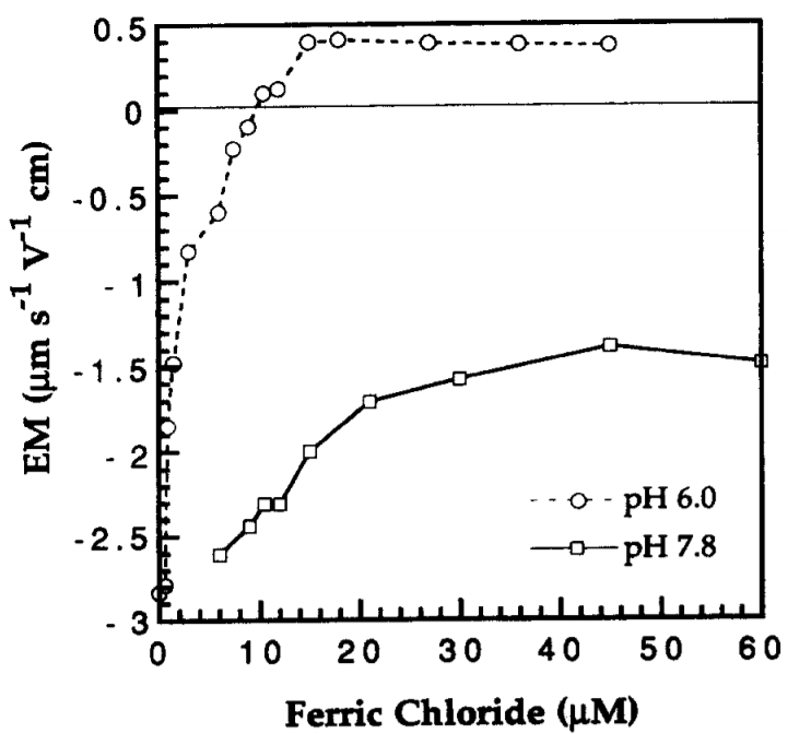
Fig. 97 Electrophoretic Mobility for final pH (after coagulant addition) of 6.0 and 7.8 as a function of \(FeCl_3\) dose
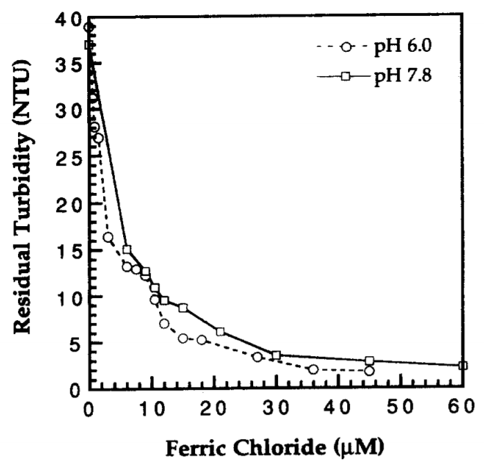
Fig. 98 The settled water turbidity was almost independent of pH even though the electrophoretic mobility was quite different for the two pH values tested.
At pH 6.0 the ferric hydroxide precipitates are positively charged and at pH 7.8 they are close to neutral. Thus it is apparent that neutralization of the clay surface charge can not explain these results.
Polymers
Synthetic polymers often made with repeating units of acrylic acid and its derivatives are used to aid flocculation by bridging between particles. For polymer bridging to occur the polymer chains must be able to span the length scale of double-layer repulsion. The thickness of the diffuse layer is about 10 nm at an ionic strength of 1 mM (Coagulants and Flocculants: Theory & Practice by Yong Kim, 1995). The length of linear polymers ranges from 100 to 1500 nm (Table 3 of Ying and Chu, 1987) and thus both synthetic polymers and coagulant nanoparticles can easily span the length scale of double-layer repulsion.
The shortest synthetic polymers are similar in size to the coagulant nanoparticles and the longest synthetic polymers are similar in length to bacteria. These polymers could create additional connections between primary particles and coagulant nanoparticles or they could connect primary particles. In either case the polymers can add connections (more bonds!) that likely have some elasticity and thus there can be more than 3 bonds connecting two particles.
Polymers undoubtedly increase the connections that bind flocs together and thus enable flocs to grow larger. The stronger flocs created by polymer addition may have unintended consequences in subsequent treatment steps. Large strong flocs are great for improved removal in plate or tube settlers. In clarifiers with floc filters they may form sludge that is more difficult to suspend after a brief shutdown. In filters it is possible that large flocs are more rigid and fail to enter the pore spaces of the filter. Thus the use of polymers may require using large media size for depth filtration. The polymers may also form mudballs in granular filters and thus require more aggressive washing.
Flocculation Theory
Particle aggregation is the fundamental mechanism that facilitates ultra low energy and low cost removal of particles and pathogens from water. Aggregation requires successful collisions. Success is defined by particles attaching when they collide.
Sticky Coagulant Nanoparticles
Prior to the AguaClara flocculation model it was widely assumed that attachment was made possible by reducing the net surface charge of the particles. The AguaClara flocculation model is based on the understanding that coagulant nanoparticles are sticky and are much larger than the length scale of the repulsive forces due to surface charges. Thus surface charge is largely irrelevant and this explains why particle aggregation begins even with very low dosages of coagulant.
Particles Follow Fluid
The collisions are caused by particles having relative motion due to fluid deformation. Particle trajectories can be different from the fluid trajectory if the density of the fluid and the particle are significantly different and if the viscous effects are small compared with inertial effects (the Stokes number). The motion of primary particles and small flocs in surface water treatment have low Stokes numbers and follow the fluid trajectory.
Long Range Transport
We need to calculate the rate of primary particle collisions. In turbulent flow flocculators the fluid deformation is caused by turbulent eddies that lose their energy to viscosity. The relative motion of particles would appear somewhat random as the small eddies have ever changing orientation and intensity. The result is that primary particles take a long meandering path before they finally approach each other and connect in a final collision. The path of relative motion prior to the collision can be thought of as having two distinct components.
The first component is long range transport when the particles are far apart with a separation distance that is proportional to the average distance between particles.
The second component is the short range transport at length scales less than the average particle separation distance to the final collision
The AguaClara flocculation model assumes a relatively high velocity and long distance random walk clearing a volume of fluid equal to the volume occupied by a single particle. This is followed by a slow, short, straight walk toward a collision. The insight that the long range transport is the rate limiting step will be used to estimate the time required for particle collisions.
Primary Particle Attachment
In our early modeling work we assumed that collisions between primary particles and large flocs were favorable. This assumption led to the prediction that the highest quality water should be obtained when the raw water has the highest turbidity. That prediction is inconsistent with observations and led to the insight that during flocculation, primary particles are only able to collide successfully with other primary particles (or potentially with other very small flocs).
The only transport mechanism that could cause a clay particle to collide with a large floc is the fluid deformation caused by the linear velocity gradient. In our flocculators that linear velocity gradient is caused by turbulent eddies at much larger scales of the flow. We hypothesize that primary particles can not attach to large flocs because primary particles can not collide with large flocs! To understand why this collision is impossible, we need a simple insight.
The insight is that the large flocs drag fluid around as they rotate (due to the linear velocity gradient). The viscous layer around the large flocs creates a flow field in which there is no location far from the flocs that will eventually approach the surface of the flocs or even approach within the clay particle radius. If this is correct, then clay particles never collide with large flocs in a linear velocity gradient flow field.
Viscous Shear Dominates
Relative velocities between particles are dominated by viscous shear because the separation distances are smaller than the inner viscous length scale. The average particle separation distance is given by
The number concentration of particles is given by
Equations (160) and (161) can be combined to obtain the relationship between separation distance and particle diameter.
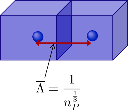
Fig. 99 The average particle separation distance is defined as the distance between centers of cubes that each contain the volume of the suspension occupied by a single particle.
Particle separation distance matters because it determines which transport mechanisms are at play when two particles approach for a collision. The particle separation distance is a function of the particle concentration. Surface water treatment plants commonly treat water with turbidity between 1 and 1000 NTU. We will first find the number of clay particles per liter in typical raw water suspensions.
Colab worksheet plotting of the number of clay particles per liter
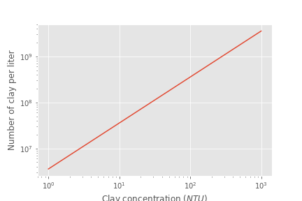
Fig. 100 Diagram of number of clay particles per liter as a function of the clay concentration. Note that even 1 NTU water has millions of primary particles per liter.
The next step is to calculate the separation distance between the clay particles over this range of clay concentrations using Equation (162).
Colab worksheet plot the separation distances
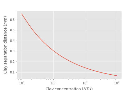
Fig. 101 The clay separation distance varies with the cube root of the concentration and thus varies over a relatively narrow range (0.07 mm to 0.7 mm) while the turbidity varies from 1 to 1000 NTU.
Given this range of particle separation distances the next question is whether transport of these particles relative to each other is driven by inertial or viscous dominated processes. Turbulent eddies devolve into smaller and smaller eddies until viscosity finally kills them. Viscosity damps out the effects of inertia at the inner viscous length scale. Higher intensity turbulence can generate more energetic small eddies and can resist the effects of viscosity longer. Thus the inner viscous length scale decreases as the turbulent energy dissipation rate increases.
The Camp-Stein velocity gradient (see Equation (46)) used for flocculators varies from about 20 to 300 Hz. We will use the inner viscous length scale, Equation (49) to determine whether viscous or inertial transport dominates particle collisions in surface water treatment given the range of particle separation distances (see Fig. 101).
Colab worksheet to plot the inner viscous length scale
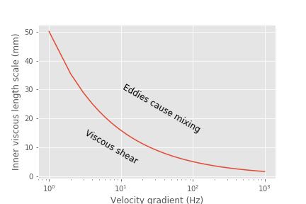
Fig. 102 The inner viscous length scale is approximately 3 to 10 mm for velocity gradients that are typically used in flocculators. Clay separation distances are smaller than the inner viscous length scale and thus viscous shear dominates particle collisions in flocculation.
By comparing Fig. 101 and Fig. 102 it is apparent that the particle separation distances commonly found in surface water treatment plants are much smaller than the inner viscous length scale for all practical flocculation velocity gradients. Thus viscosity will dominate the flocculation process. This key insight reveals why turbulent flow flocculators have been designed using the dimensionless grouping \(G \theta\) which is fundamentally \(\sqrt\frac{\epsilon}{\nu} \theta\). Given that flocculation is viscous dominated implies that the flocculation process will slow down as the temperature increases and the viscosity increases.
The flocculation model (see Equation (177)) reveals that the velocity gradient multiplied by the residence time in the flocculator will determine the final spacing between the primary particles. Our goal is to maximize the spacing between particles and thus to minimize the number of particles and potential pathogens in our drinking water.
There are diminishing returns on investment in larger flocculators to produce cleaner water because the time between collisions increases as the primary particles are spaced further apart. Eventually other processes including fluidized floc filters (floc filters), plate settlers, and sand-floc filter (stacked rapid sand filter) are able to reduce the primary particle concentration at a lower cost.
Collision Potential, \(\tilde{G} \theta\), and Energy Dissipation Rate, \(\varepsilon\)
Collision potential \((\tilde{G} \theta)\) represents the number of potential particle collisions in a volume of fluid. It is a dimensionless parameter which is a logical design parameter for flocculators; large \(\tilde{G} \theta\) values indicate lots of collisions (good) while small values indicate fewer collisions (not so good). AguaClara flocculators usually aim for a collision potential of \((\tilde{G} \theta) = 37,000\), which has worked well in AguaClara plants historically. However, this value may change as research continues. The value for collision potential is obtained by multiplying \(\tilde{G}\), a parameter for average fluid shear with units of \(\frac{1}{[T]}\), and \(\theta\) , the residence time of water in the flocculator, with units of :\([T]\) . \(\theta\) is intuitive to measure, calculate, and understand. \(\tilde{G}\) is a bit more difficult.
In any control volume or reactor, the total energy dissipated is equal to the mechanical energy that is converted to heat, \(g h_L\). The amount of time required to dissipate that energy is the residence time of the water in the reactor, \(\theta\).
Note that the equation above is for \(\bar \varepsilon\), not \(\varepsilon\). Since the head loss term we are using, \(h_L\), occurs over the entire reactor, it can only be used to find an average energy dissipation rate for the entire reactor. Combining the equations above, \(G = \sqrt{\frac{\varepsilon}{\nu}}\) and \(\bar \varepsilon = \frac{g h_L}{\theta}\), we can get an equation for \(\tilde{G}\) in terms of easily measurable parameters:
We can use this to obtain a final equation for collision potential of a reactor:
Note: When we say \(G \theta\) we are almost always referring to \(\tilde{G} \theta\).
The head loss for a flocculator can be estimated quickly based on the basis of design values of \(\tilde{G} \theta\) and \(\tilde{G}\). Rearrange Equation (164) to obtain
The head loss increases with the required collision potential \(\tilde{G} \theta\) and it also increases with the velocity gradient. Cold water also requires more head loss due to the increased viscosity and hence more energy is required to deform the fluid and achieve the target collision potential.
Generating Head Loss with Baffles
What are Baffles?
Now that we know how to measure collision potential with head loss, we need a way to actually generate head loss. While both major or minor losses can be the design basis, it generally makes more sense to use major losses only for very low-flow flocculation (lab-scale) and minor losses for higher flows, as flocculation with minor losses tends to be more space-efficient. Since this book focuses on town and village-scale water treatment (5 L/S to 120 L/S), we will use minor losses as our design basis.
To generate minor losses, we need to create flow expansions. AguaClara does this with baffles, which are obstructions in the channel of a flocculator to force the flow to switch directions by 180°. Baffles in AguaClara plants are plastic sheets, and all of the baffles in one flocculator channel are connected to form a baffle module. Fig. 103 shows an AguaClara flocculator and Fig. 104 shows the assembly of a baffle module.
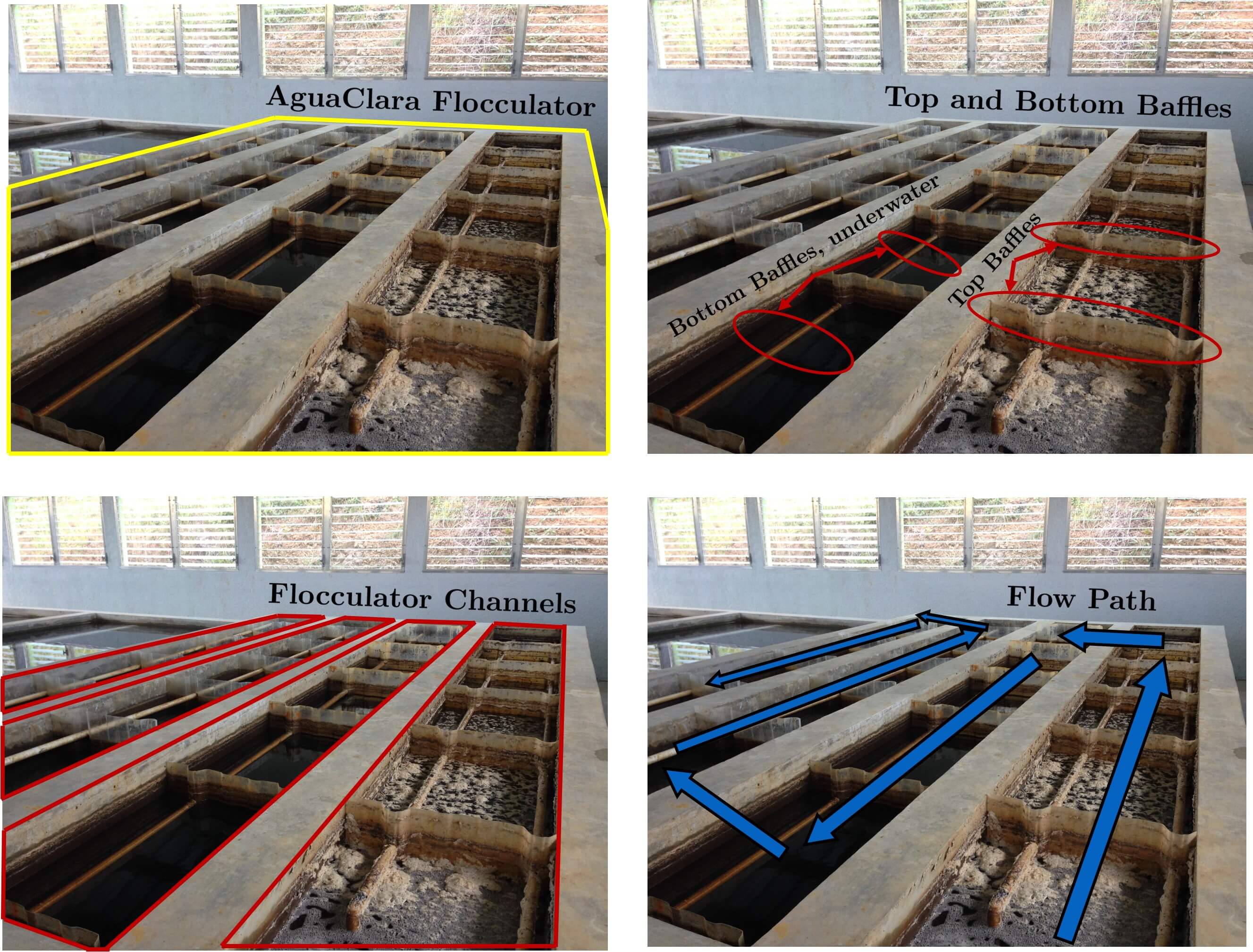
Fig. 103 Clockwise from the top left the images show: the outline of the entire flocculator, some top and bottom baffles in the channels, the 4 flocculator channels in this flocculator, and the flow path of water through the flocculator
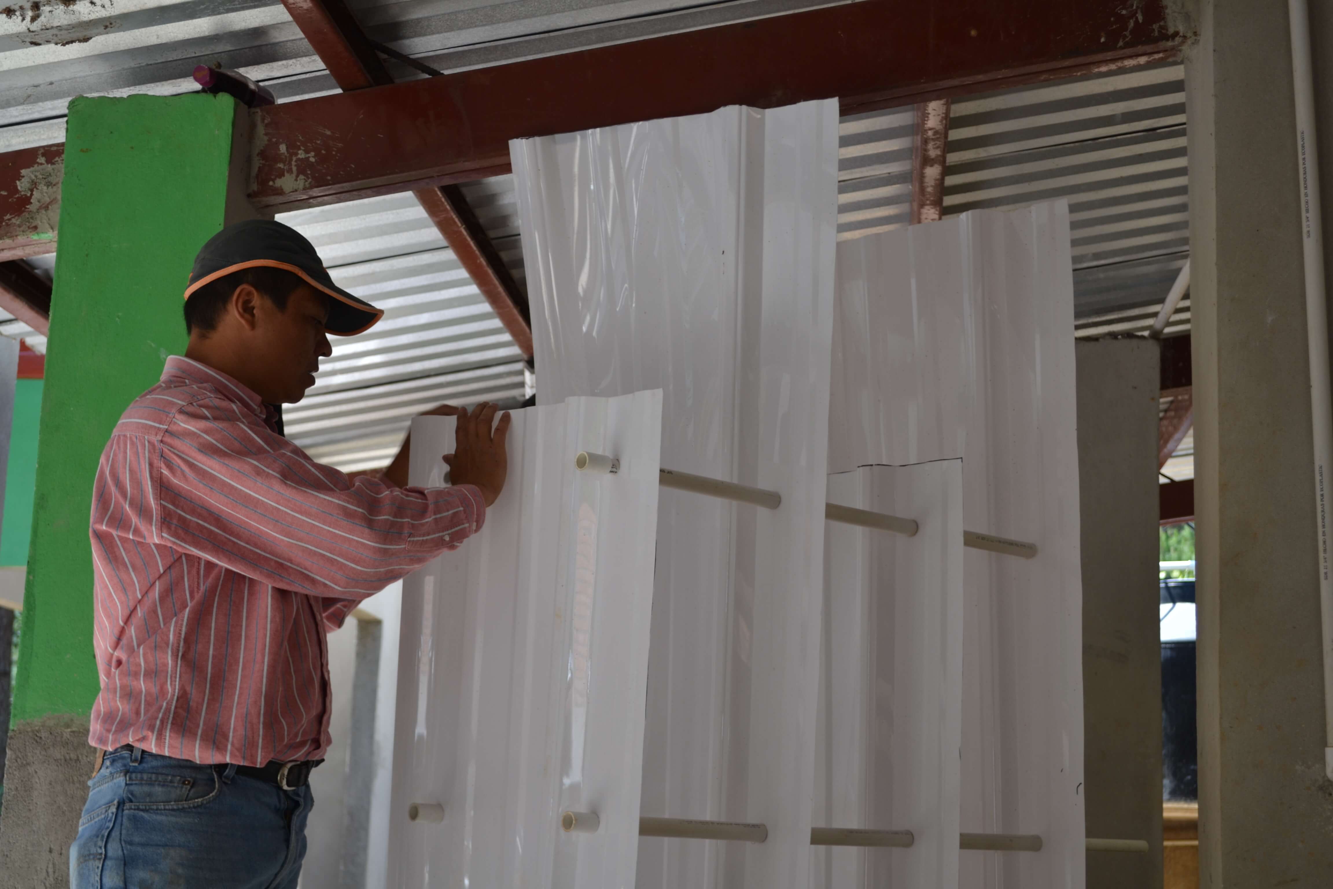
Fig. 104 Before being inserted into the flocculator channel, the baffle module is constructed as a unit as shown above.
AguaClara flocculators, like the one pictured above, are called horizontal vertical flow flocculators (see Fig. 113).
Finding the Minor Loss of a Baffle
Before beginning this section, it is important to understand how water flows through a baffled flocculator. This flow path is shown in Fig. 105. Take note of the thin red arrows; they indicate the compression of the flow around a baffle.
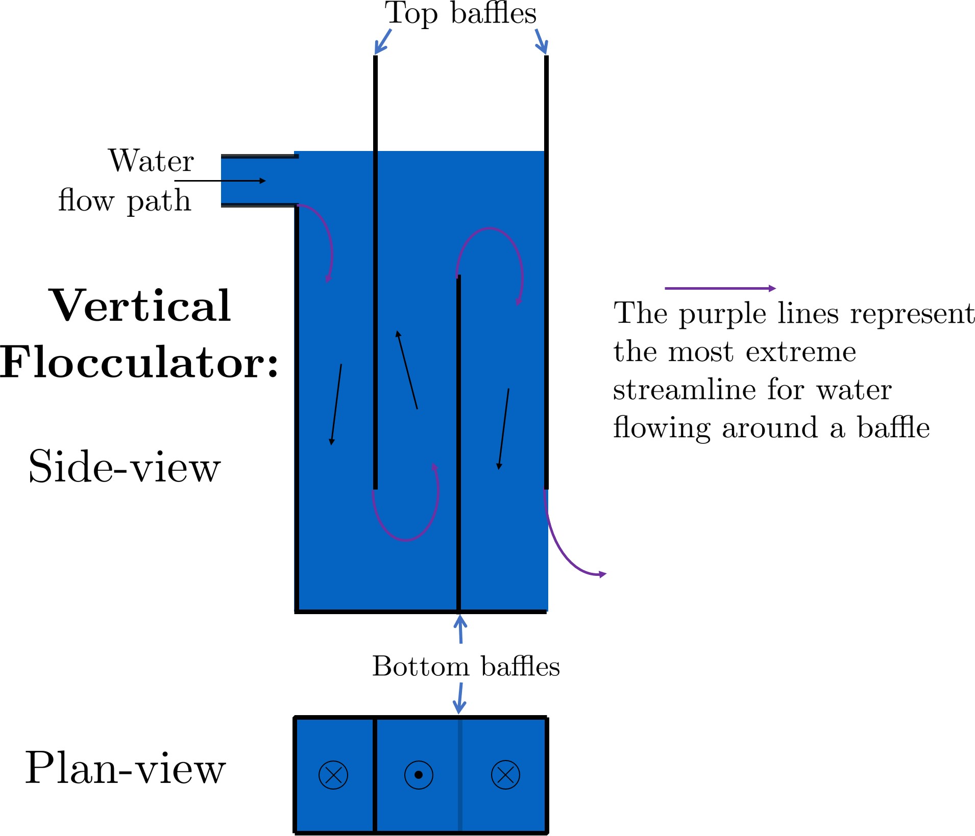
Fig. 105 Flow path through a vertical flow hydraulic flocculator
Since baffles are the source of head loss via minor losses, we need to find the minor loss coefficient of one baffle if we want to be able to quantify its head loss. To do this, we apply fluid mechanics intuition and check it against a computational fluid dynamics (CFD) simulation. Flow around a 90° bend has a vena contracta value of \(\Pi_{vc} = 0.611\) as given by Equation (14). Flow around a 180° bend therefore has a value of \(\color{red}{\Pi_{vc}^{baffle} = \Pi_{vc}^2 = 0.373}\). This number is roughly confirmed with CFD, as shown in the image below.
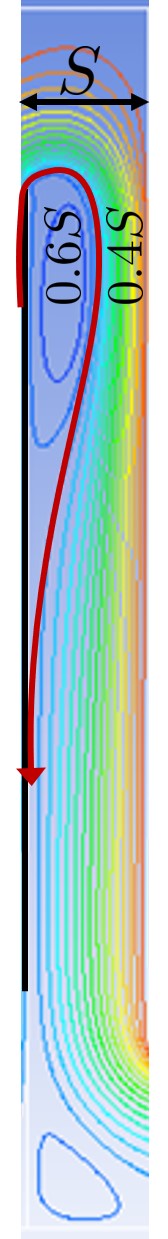
Fig. 106 The 180° bend at the end of a baffle results in a dramatic flow contraction with all of the flow passing through less than 40% of the space between the baffles.
We can therefore state with reasonable accuracy that, when most contracted, the flow around a baffle goes through 37.3% of the area it does when expanded, or \(A_{contracted} = \Pi_{vc}^{baffle} A_{expanded}\). Through the :ref:`third form of the minor loss equation <heading_minor_losses>, \(h_e = K \frac{\bar v_{out}^2}{2g}\) and its definition of the minor loss coefficient, \(K = \left( \frac{A_{out}}{A_{in}} -1 \right)^2\), we can determine the minimum minor loss coefficient for flow around a single baffle:
This \(K_{baffle_{min}}\) has been used to design flocculators in AguaClara plants until 2021. The plant at Gracias revealed that the observed head loss was greater than predicted. This paper by Haarhoff in 1998 (DOI: 10.2166/aqua.1998.20), the \(K_{baffle}\) values found are context dependent and empirically based. Further analysis of how \(K_{baffle}\) varies with the geometry of the flocculator is given in the section on Baffle Minor Loss Coefficient.
Equation (166) doesn’t account for the fact that for a series of baffles (or flow contractions) the flow might not be able to fully expand before entering the next baffle (or contraction). The distance required for the contracted flow to expand can be estimated from jet equations (see section on Baffle Minor Loss Coefficient for an estimate of how the minor loss coefficient increases when the flow doesn’t fully expand).
Flocculator Efficiency
When designing an effective and efficient flocculator, there are two main problems that we seek to avoid:
Having certain sections in the flocculator with such high local \(\tilde{G}\) values that our big, fluffy flocs are sheared apart into smaller flocs.
Having dead space. Dead space means volume within the flocculator that is not being used to facilitate collisions. Dead space occurs after the flow has fully expanded from flowing around a baffle and before it reaches the next baffle.
Fortunately for us, both problems can be quantified with a single ratio:
High values of \(\Pi_{\tilde{G}}^{G_{max}}\) occur when one or both of the previous problems is present. If certain sections in the flocculator have very high local \(G\) values, then \(G_{max}\) becomes large. If the flocculator has a lot of dead space, then \(\tilde{G}\) becomes small. Either way, \(\Pi_{\tilde{G}}^{G_{max}}\) becomes larger.
Note: Recall the relationship between \(G\) and \(\varepsilon\) : \(G = \sqrt{ \frac{\varepsilon}{\nu} }\). From this relationship, we can see that \(G \propto \sqrt{\varepsilon}\). Thus, by defining \(\Pi_{\tilde{G}}^{G_{max}}\), we can also define a ratio for max to average energy dissipation rate:
Therefore, by making our \(\Pi_{\tilde{G}}^{G_{max}}\) as small as possible, we can be sure that our flocculator is efficient, and we no longer have to account for the previously mentioned problems. A paper by Haarhoff and van der Walt in 2001 (DOI: 10.2166/aqua.2001.0014) uses CFD to show that the minimum \(\Pi_{\tilde{G}}^{G_{max}}\) attainable in a hydraulic flocculator is \(\Pi_{\tilde{G}}^{G_{max}} = \sqrt{2} \approx 1.4\), which means that \(\Pi_{\bar \varepsilon}^{\varepsilon_{max}} = \left( \Pi_{\tilde{G}}^{G_{max}} \right)^2 \approx 2\). So how do we optimize an AguaClara flocculator to make sure \(\Pi_{\tilde{G}}^{G_{max}} = \sqrt{2}\)?
We define and optimize a performance metric:
Where \(H_e\) is the distance between flow expansions in the flocculator and \(S\) is the spacing between baffles. For now, \(H_e\) is approximated as the height of water in the flocculator.
Since \(G_{max}\) is determined by the fluid mechanics of flow around a baffle, our main concern is eliminating dead space in the flocculator. We do this by placing an upper limit on \(\frac{H_e}{S}\). To determine this upper limit, we need to find the distance it takes for the flow to fully expand after it has contracted around a baffle.
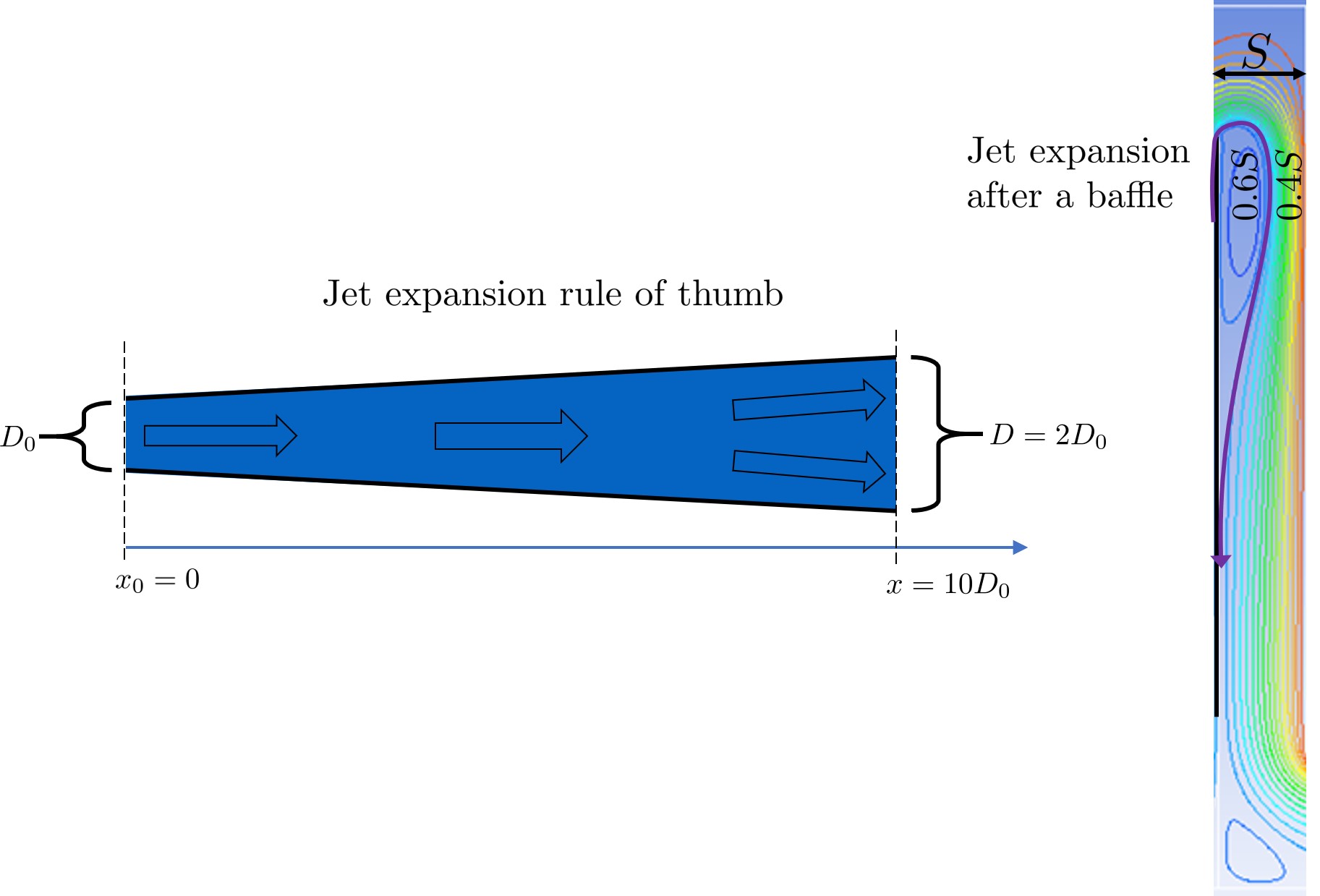
Fig. 107 A turbulent jet expands in width by approximately one unit for every 10 units downstream (see Equation (186)).
Using the equation and image above, we can find the distance required for the flow to fully expand around a baffle as a function of baffle spacing \(S\). We do this by substituting \(D_{cp} = (0.373 S)\) along with \(D = S\) to approximate how much distance, \(x = L_{jet}\), the contracted flow has to cover.
where \(\Pi_{BaffleJet_{exp}}\) is the dimensionless rate of expansion for the jet that has a baffle on one side.
This gives a rough estimate of the maximum distance between flow expansions while ensuring that there are no zones of low turbulence in the flocculator. The relationship between \(L_{jet_{max}}\) and the flocculator geometry is given in Equation (188).
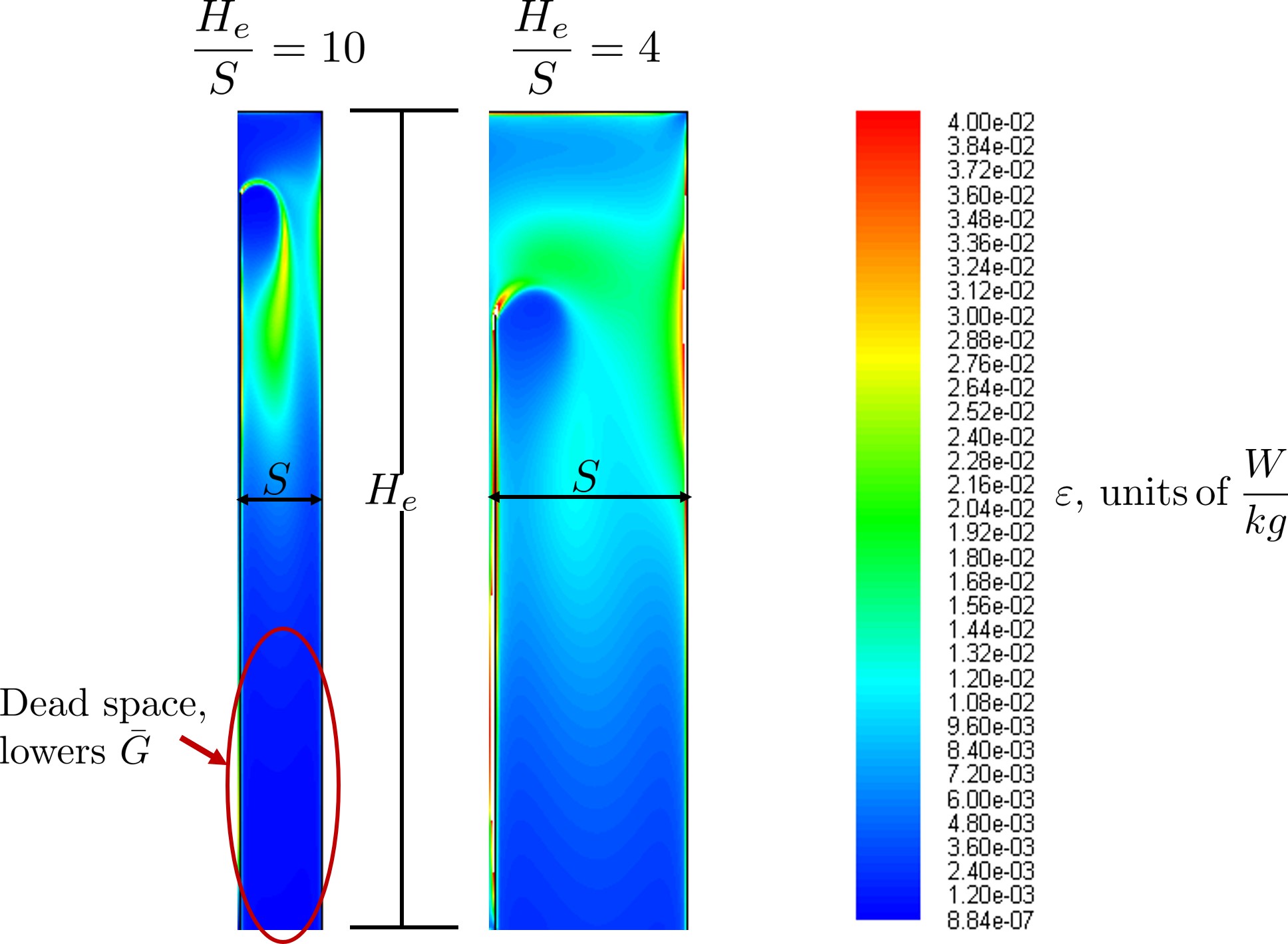
Fig. 108 High \(\frac{H_e}{S}\) ratios result in flocculator zones with low velocity gradients that don’t contribute effectively.
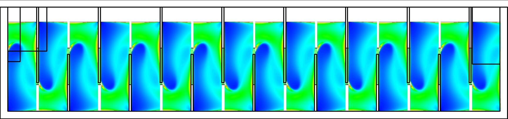
Fig. 109 Each bend creates a flow contraction and when the flow expands it converts kinetic energy into turbulent eddies and fluid deformation. The fluid deformation is what ultimately creates collisions between particles.
The lowest functional \(\frac{H_e}{S}\) ratio, \(\Pi_{H_eS_{min}}\) is an important constraint for the design of flocculators that have vertical flow between baffles because it sets the minimum water depth in the flocculator channel. The absolute minimum value of \(\frac{H_e}{S}\) is set by the flow geometry to ensure that water can’t flow straight through the flocculator without going back and forth or up and down around the baffles. This short circuiting would depend on the slot width, defined below.
Slot width is the distance between the water level and the top of an upper baffle (which is the same distance between the flocculator floor and the bottom of an upper baffle). This distance is referred to as the slot width (Haarhoff 1998) DOI: 10.2166/aqua.1998.20”) and is defined by the slot width ratio, which describes the slot width as a function of baffle spacing \(S\). Slot width is shown in the following image:
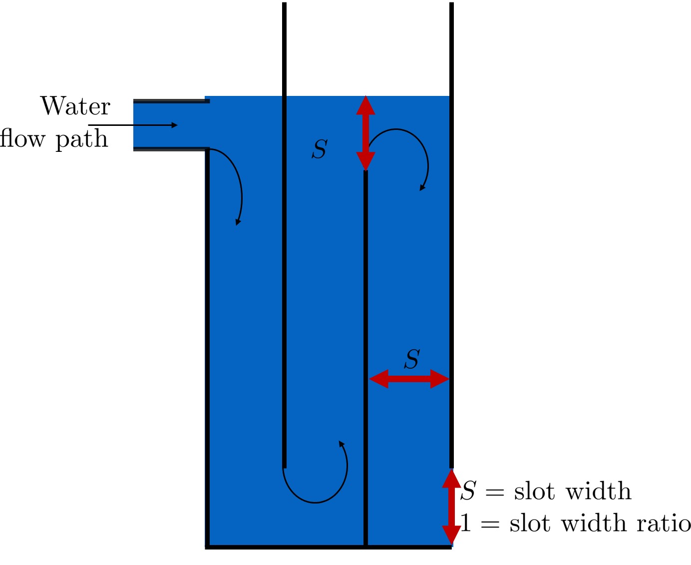
Fig. 110 The space between the bottom of the upper baffle and the floor of the flocculator is defined as the slot width.
AguaClara uses a slot width ratio of 1 for its flocculators. This number has been the topic of much hydraulic flocculation research, and values between 1 and 1.5 are generally accepted for hydraulic flocculators. See the following paper and book respectively for more data on slot width ratios and other hydraulic flocculator parameters: [Haa98], [SO84]. We base our slot width ratio of 1 on research done by [HvdW01] on optimizing hydraulic flocculator parameters to maximize flocculator efficiency.
The minimum \(\Pi_{H_eS}\) allowable depends on the slot with ratio. If \(\Pi_{H_eS}\) is less than twice the slot width ratio, the water would flow straight through the flocculator without having to bend around the baffles. This means that the flocculator would not be generating almost any head loss, and the top and bottom of the flocculator will largely be dead space. See the following image for an example:
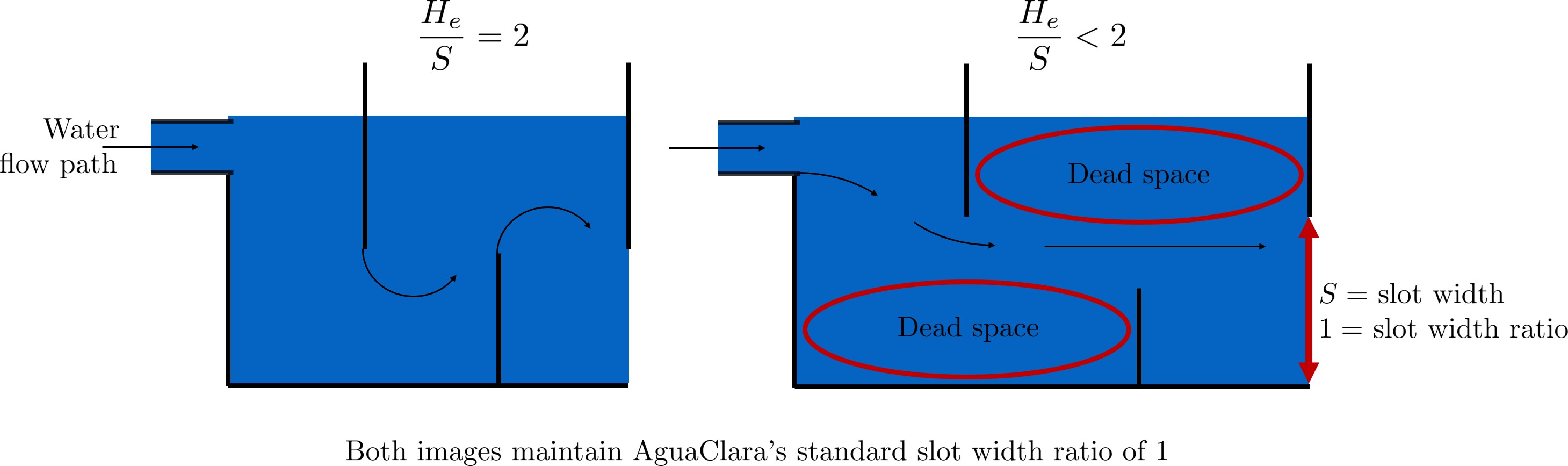
Fig. 111 The minimum \(\frac{H_e}{S}\) ratio is set by the need to prevent short circuiting through the flocculator.
Thus, \(\Pi_{H_eS_{min}}\) should be at least twice the slot width ratio, \(\Pi_{H_eS_{min}} = 2\). Historically, AguaClara plants have been designed using \(\Pi_{H_eS_{min}} = 3\). This adds a safety factor of sorts, ensuring that the flow does not short-circuit through the flocculator and also allowing more space for the flow to expand after each contraction.
Although this value of \(\Pi_{H_eS}\) meets the geometric constraints it is not necessarily the best design since the flow doesn’t come close to fully expanding between contractions. This results in a much higher baffle loss coefficient and a higher level of uncertainty of the exact value of that loss coefficient. Thus we recommend using higher values of \(\Pi_{H_eS}\) when possible.
Flocculator Geometry
The geometry of hydraulic flocculators changes rather dramatically as the flow rate increases from a fraction of a L/s up to thousands of L/s. The transition from one geometry to another is dependent on economic factors, fabrication constraints, and integration with the rest of the plant design. Thus the flow transition between each of the distinct geometries will evolve as design optimization progresses. Flows between 0.5 L/s and 20 L/s are efficiently handled by a Vertical-Horizontal flow flocculator as shown in Fig. 112.
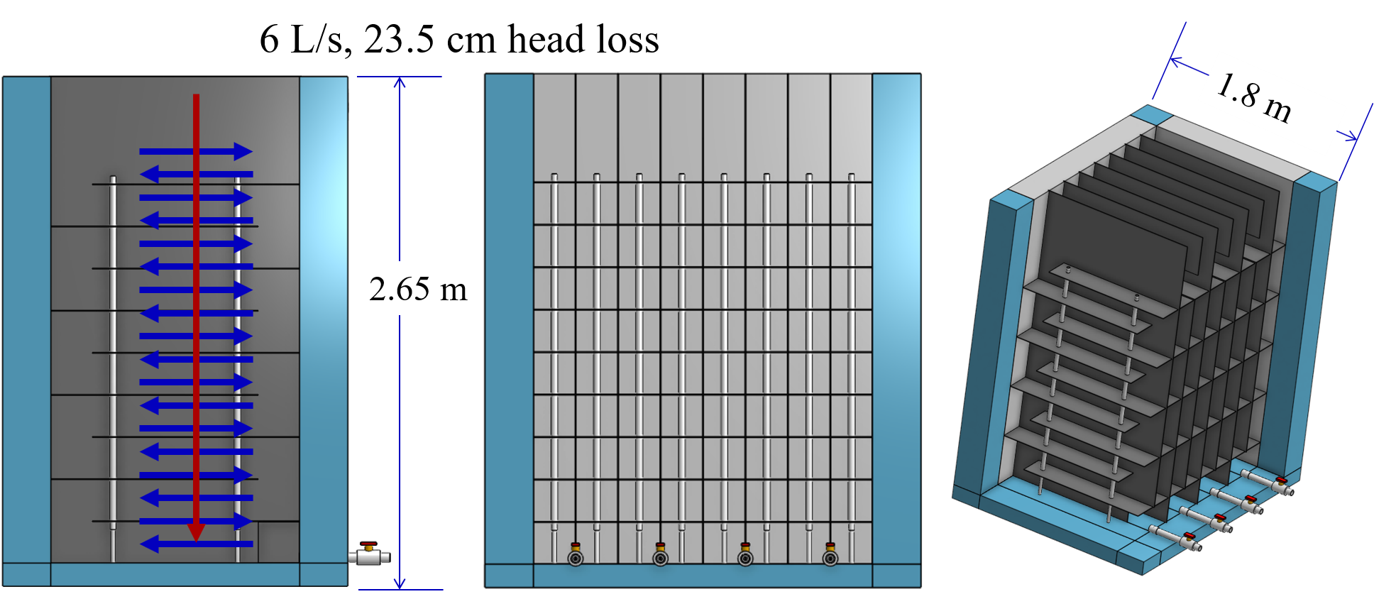
Fig. 112 The vertical-horizontal flocculator has vertical flow in the channels and horizontal flow between baffles. This design is for 6 L/s with 23.5 cm of head loss.
As the flows increase the spacing between baffles grows larger and a vertical-horizontal flocculator would need to be very deep in order to accommodate a reasonable number of baffle spaces per channel. The geometry switches to horizontal-vertical for flows between about 20 and 200 L/s as shown in Fig. 113.
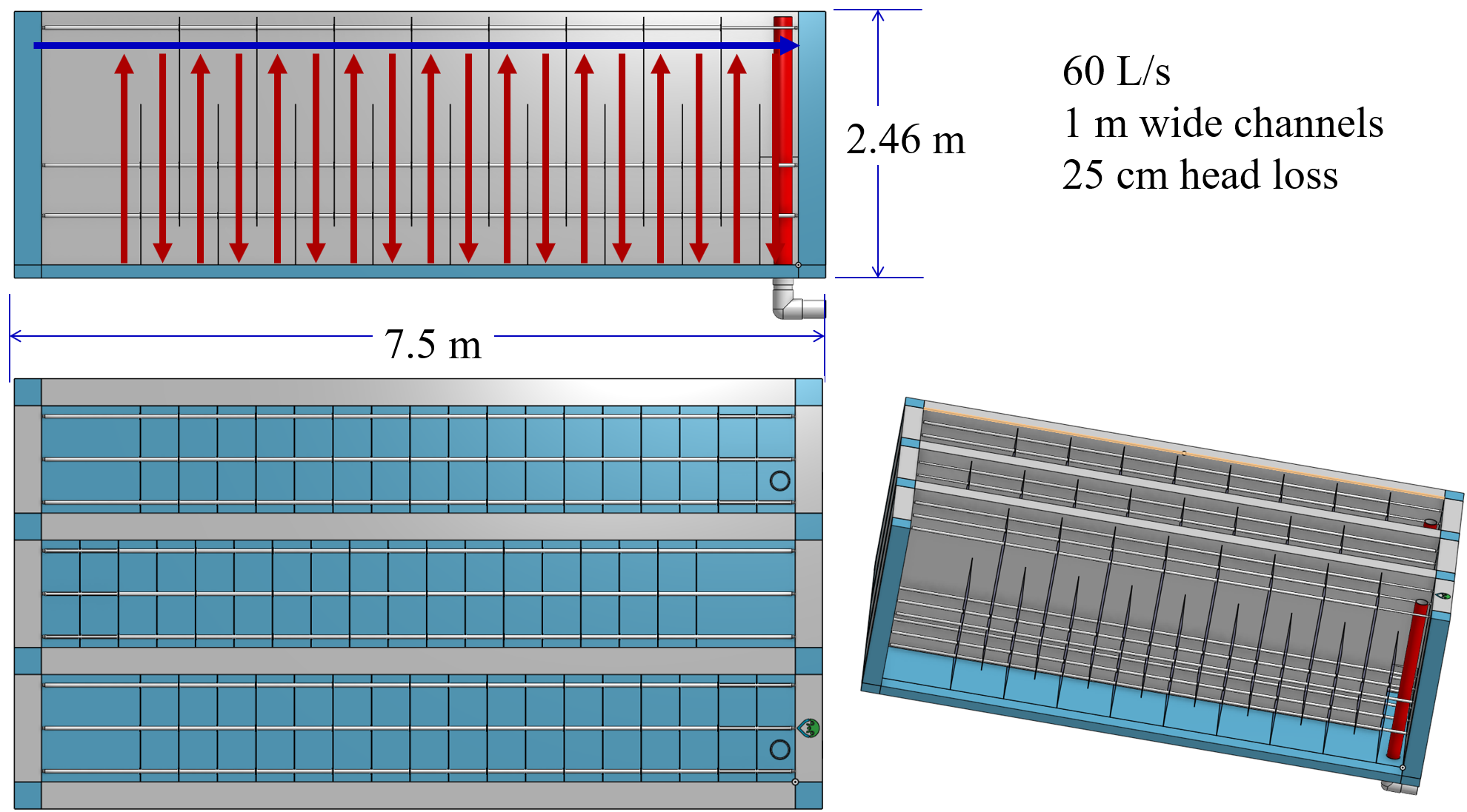
Fig. 113 The horizontal-vertical flocculator has horizontal flow in the channels and vertical flow between baffles.This design is for 60 L/s with 1 m wide channels and 25 cm of head loss.
As the flow increases above 200 L/s the required depth to accommodate a reasonable H/S ratio will exceed the desired depth (from a construction and maintenance perspective) and the optimal design will switch to a horizontal-horizontal flocculator as shown in Fig. 114.
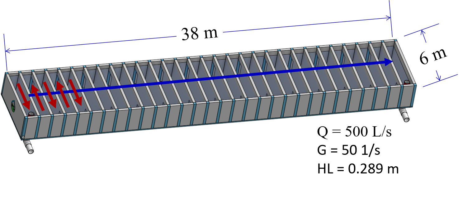
Fig. 114 The horizontal-vertical flocculator has horizontal flow in the channels and vertical flow between baffles. This design is for a 500 L/s flow with 29 cm of head loss. The channels are 2.6 m deep.