Python Tutorial

Table 27 Code resources.
Description	Theme	Example function	Function call
Python functions	low level programming functions	open a file	open(file, mode=’r’)
Pint universal constants	physical constants with units	Avogadro’s number	u.avogadro_number
Pint units	units that can be attached to numbers and numpy arrays	5 m/s	5* u.mm/u.s
aguaclara.core. physchem	pipeflow, orifices, viscosity of water, weirs, manifolds, Kozeny equation	total head loss in a straight pipe	headloss(FlowRate, Diam, Length, Nu, PipeRough, KMinor)
aguaclara.research. floc_model	AguaClara flocculation model, velocity gradients, Kolmogorov length scales	velocity gradient in a coiled tube	g_coil(FlowPlant, IDTube, RadiusCoil, Temp)
aguaclara.research. environmental_processes_analysis	carbonate system, CMFR and advection dispersion reactor analysis	extract data from ProCoDA generated Gran analysis file	Gran(data_file_path)
aguaclara.research. procoda_parser	Extracts data from multiple ProCoDA files based on the state and data column	extract a column of data from a ProCoDA data file	column_of_data (data_file_path, start, column)
SciPy	computing integrals numerically, solving differential equations, optimization, and sparse matrices	root finding	root(func, 0.3)
NumPy	Array manipulation and math functions	create an array with linearly spaced elements	np. linspace (start,stop,num)
PyPlot	Graphs!	Create beautiful graphs	see below

Import statements

import aguaclara as ac
from aguaclara.core.units import unit_registry as u
import numpy as np
import matplotlib.pyplot as plt
import pandas as pd
from scipy import constants, interpolate

Hint: If you are typing a function name and want to know what the options are for completing what you are typing, just hit the tab key for a menu of options.

Hint: If you want to see the source code associated with a function, you can do the following import inspect inspect.getsource(foo)

Where “foo” is the function that you’d like to learn about.

Markdown

Markdown allow you to mix code, beautiful Latex equations, nicely formatted text, figures, and tables.

\[c = \sqrt{a^2 + b^2}\]

Markdown does not handle automatic numbering of equations, figures, and tables.

The Python Kernel remembers all definitions (functions and variables) as they are defined based on execution. Thus if you fail to execute a line of code, the parameters defined in that line won’t be available. Similarly, if you define a parameter and then delete that line of code, that parameter remains defined until you reset all runtimes or restart.

Before submitting a file for others to use, you need to verify that all of the dependencies are defined and that you didn’t accidently delete a definition that is required. You can do this by resetting all runtimes (Runtime menu) and then running all.

Transitioning From Matlab To Python

Indentation - When writing functions or using statements, Python recognizes code blocks from the way they are indented. A code block is a group of statements that, together, perform a task. A block begins with a header that is followed by one or more statements that are indented with respect to the header. The indentation indicates to the Python interpreter, and to programmers that are reading the code, that the indented statements and the preceding header form a code block.

Suppressing Statements - Unlike Matlab, you do not need a semi-colon to suppress a statement in Python;

Indexing - Matlab starts at index 1 whereas Python starts at index 0.

Functions - In Matlab, functions are written by invoking the keyword “function”, the return parameter(s), the equal to sign, the function name and the input parameters. A function is terminated with “end”.:

function
  y = average(x)
  if ~isvector(x)
    error('Input must be a vector') end
    y = sum(x)/length(x);
    end

In Python, functions can be written by using the keyword “def”, followed by the function name and then the input parameters in parenthesis followed by a colon. A function is terminated with “return”.:

def average(x):
  if ~isvector(x)
  raise VocationError("Input must be a vector")
  return sum(x)/length(x)

Statements - for loops and if statements do not require the keyword “end” in Python. The loop header in Matlab varies from that of Python. Check examples below:

Matlab code:

s = 10;
H = zeros(s);
  for c = 1:s
    for r = 1:s
    H(r,c) = 1/(r+c-1);
    end
  end

Printing - Use “print()” in Python instead of “disp” in Matlab.

Helpful Documents

Numpy for Matlab Users

Stepping from Matlab to Python

Python for Matlab Users, UC Boulder

Units

Engineering requires calculations with units. Prior to modern computer languages engineers used paper and pencil, slide rules, calculators, and more recently spreadsheets to do calculations. All of these methods are prone to calculation errors because units aren’t handled as an essential part of each value. Spreadsheets are especially notorious for calculation errors because unit conversions are buried in formulas that are hidden in the cells.

Operations on values with units follow very clear algebraic rules and thus units can be attached to numerical values and carried through math operations. This capability is implemented in Python using Pint . The Pint package includes a host of units and prefixes (such as \(\mu\) for \(10^{-6}\)). As you master using Python and Pint you will say goodbye to mindless unit conversions forever!

Environmental engineers historically described surface loading rates for clarifiers using units of gal/min per square foot. How fast is \(\frac{1 gpm}{ft^2}\) in \(\frac{mm}{s}\)?

V_surface_loading_rate = (1 * u.gal/(u.min * u.ft**2)).to(u.mm/u.s)
print('The surface loading rate is', V_surface_loading_rate)
print('The surface loading rate is', ac.round_sig_figs(V_surface_loading_rate,2))

The surface loading rate is 0.6791 millimeter / second

After reducing the number of significant digits to 2 we obtain: The surface loading rate is 0.68 millimeter / second

How long does it take to stop a car that is initially traveling at 60 mph if the coefficient of friction is 0.5?

v_0 = 60 * u.mile/u.hr
friction_coefficient = 0.5
deceleration = friction_coefficient * u.standard_gravity
t_deceleration = v_0/deceleration
print('The time to stop the car is',t_deceleration)
print('The time to stop the car is',t_deceleration.to_base_units())

The time to stop the car is 120 mile / hour / standard_gravity

We add the .to_base_units() directive to force pint to simplify the units.

The time to stop the car is 5.47 second

Many functions written in Python do not yet handle units and thus it is sometimes necessary to remove the units. Examples include graphs (althougth units might be coming to matplotlib), SciPy functions, and the NumPy functions used to populate arrays. For these cases you can strip the units off a number using the .magnitude method. Be careful to make sure you know what the units are before you remove them otherwise you may be confused by the results!

Q = 5 * u.gal/u.min
fill_time = 3*u.hr
Volume = Q * fill_time
print('The volume is',Volume)
print('The magnitude of the Volume is', Volume.magnitude)
print('The units of the flow are', Volume.units)
#force pint to display in a selected set of Units
print('The volume is',Volume.to(u.kL))

The volume is 15 gallon * hour / minute

The magnitude of the Volume is 15.0

The units of the flow are gallon * hour / minute

The volume is 3.41 kiloliter

It is useful to force pint to display the result in the units of your choice.

Arrays and units

Use NumPy arrays rather than Python lists to enable math with numbers and units. When creating arrays with units remember that

Array elements don’t have units!

Arrays can have units.

Therefore always attach units to the array after the array has been created. This means that array elements should be dimensionless and thus arrays must be created using dimensionless values.

We can use NumPy linspace with a simple change to make it dimensionless. Usually linspace has start and stop elements that would logically have units: np.linspace(start, stop, num). But elements can’t have units! We can make the inputs to linspace be dimensionless to create a dimensionless array and then multiplies it by the final value that includes the units to scale the array correctly. For evenly spaced arrays starting at the end of the first space we have either:

np.linspace(start/stop, 1, num) * stop

np.linspace(1 / num, 1, num) * stop

For evenly spaced arrays starting with zero we have:

np.linspace(0, 1, num+1) * stop!

The print function can’t currently handle arrays with units. The array can be printed nicely in two steps as shown below.

n_rows = 10
Flow = 20 * u.L/u.s
Flow_array = (np.linspace(1 / n_rows, 1,n_rows) * Flow)
print('The array of flow rates is',Flow_array.magnitude,Flow_array.units)

Flow_array = (np.linspace(1 / n_rows, 1,n_rows) * Flow).to(u.L/u.s)
print('The array of flow rates is',Flow_array.magnitude,Flow_array.units)

Flow_array = (np.linspace(0, 1,n_rows+1) * Flow).to(u.L/u.s)
print('The array of flow rates is',Flow_array.magnitude,Flow_array.units)

[ 2. 4. 6. 8. 10. 12. 14. 16. 18. 20.] liter / second

Plotting

We will use this pyplot coding style .

fig is a Figure instance—like a blank canvas

ax is an AxesSubplot instance—think of a frame for plotting in

Create a graph showing flow rate vs depth for two linear flow orifice meters that have a depth range of 20 cm and flow ranges of 50 and 70 L/s.

Legend location options

Colors

‘b’, ‘g’, ‘r’, ‘c’, ‘m’, ‘y’, ‘k’, ‘w’

blue, green, red, cyan, magenta, yellow, black, white

Data markers (if you are plotting data and not a model or curve fit)

H_max = 20 * u.cm
Q_max1 = 50 * u.L/u.s
Q_max2 = 70 * u.L/u.s
num = 50
a = np.linspace(0, 1, num)
x = a * H_max
y = np.empty( (2,num) )
y1 = a * Q_max1
y2 = a * Q_max2

fig, ax = plt.subplots()
ax.plot(x, y1, 'r-', linewidth=2, label=Q_max1, alpha=0.6)
ax.plot(x, y2, 'b-', linewidth=2, label=Q_max2, alpha=0.6)

ax.set(xlabel='water depth ('+str(x.units) +')')
#ax.set(ylabel='Flow rate ('+str(Q_max1.units)+')')
#Below is the method for using latex to format the units
ax.set(ylabel='Flow rate ' + r'$\left (\frac{L}{s}\right )$')

# options: linear or log
ax.set(yscale='log')
ax.set(xscale='linear')

ax.grid(True)

#options:
ax.legend(loc='best')

#alternative method to create a legend instead of using "label=Q_max1 in ax.plot"
#ax.legend([Q_max1,Q_max2])

fig.savefig('../Images/LFOM_flow_vs_height')
plt.show()

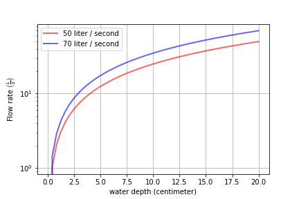
LFOM flow vs height — Fig. 245 The flow through an LFOM is directly proportional to the height of the water above the bottom of the first row of orifices.

Indexing is done by row and then by column. To call all of the elements in a row or column, use a colon. As you can see in the following example, indexing in python begins at zero. So a[:,1] is calling all rows in the second column

#create an empty array
a = np.empty((2,5))
np.shape(a)
np.size(a)
#Given that I'm going to using np.array to assign the elements I didn't need to create the empty array first.
a = np.array([[1,2,3,4,5], [2,4,6,8,10]])
a[1,3]
a[0]
a[1]
a[:,2]
#access the last row by find the shape, selecting the 2nd element in the shape, and then subtracting one
a[:,np.shape(a)[1]-1]
'''specify a range of values in an array. Use a colon to slice the array, with the number before the colon being the index of the first element, and the number after the colon being **one greater** than the index of the last element'''
a[0,2:5]

Example problem

Calculate the number of moles of methane in a 20 L container at 15 psi above atmospheric pressure with a temperature of 30 C.

# First assign the values given in the problem to variables.
P = 15 * u.psi + 1 * u.atm
T = 30 * u.degC
V = 20 * u.L
# Use the equation PV=nRT and solve for n, the number of moles.
# The universal gas constant is available in pint.
nmolesmethane = (P*V/(u.R*T.to(u.kelvin))).to_base_units()
print(nmolesmethane)
print('There are ', nmolesmethane ,' of methane in the container.')

There are 1.625 mole of methane in the container.

Functions

When it becomes necessary to do the same calculation multiple times, it is useful to create a function to facilitate the calculation in the future.

Function blocks begin with the keyword def followed by the function name and parentheses ( ).

Any input parameters or arguments should be placed within these parentheses.

The code block within every function starts with a colon (:) and is indented.

The statement return [expression] exits a function and returns an expression to the user. A return statement with no arguments is the same as return None.

(Optional) The first statement of a function can the documentation string of the function or docstring, written with apostrophes .

Below is an example of a function that takes three inputs, pressure, volume, and temperature, and returns the number of moles.

# Creating a function is easy in Python
def nmoles(P,V,T):
    return (P*V/(u.R*T.to(u.kelvin))).to_base_units()

Try using the new function to solve the same problem as above. You can reuse the variables. You can use the new function call inside the print statement.

print('There are', nmoles(P,V,T),'of methane in the container.')

There are 1.62 mol of methane in the container.

Pipe Database

The pipes has many useful functions concerning pipe sizing. It provides functions that calculate actual pipe inner and outer diameters given the nominal diameter of the pipe. Note that nominal diameter just means the diameter that it is called (hence the discriptor “nominal”) and thus a 1 inch nominal diameter pipe might not have any dimensions that are actually 1 inch!

import aguaclara.core.pipes as pipe
# The OD function in pipedatabase returns the outer diameter of a pipe given the nominal diameter, ND.
pipe.OD(6*u.inch)

6.625 inch

The ND_SDR_available function returns the nominal diameter of a pipe that has an inner diameter equal to or greater than the requested inner diameter SDR, standard diameter ratio . Below we find the smallest available pipe that has an inner diameter of at least 7 cm

IDmin = 7 * u.cm
SDR = 26
ND_my_pipe = ac.ND_SDR_available(IDmin,SDR)
ND_my_pipe

3.0 inch

The actual inner diameter of this pipe is

ID_my_pipe = ac.ID_SDR(ND_my_pipe,SDR)
print(ID_my_pipe.to(u.cm))

8.2 cm

We can display the available nominal pipe sizes that are in our database.

ac.ND_all_available()