Fluid Mechanics
This chapter is meant to be a refresher on fluid mechanics. It will only cover the topics in fluids mechanics that will be used heavily in the course.
If you wish to review fluid mechanics in (much) more detail, please refer to this guide. Note that to view this link, you will need a Github account. If you wish to review from a textbook, you can find a pdf of a good fluid mechanics textbook by Frank White here.
Introductory Concepts
Before diving in to the rest of this document, there are a few important concepts to focus on which will be the foundation for building your understanding of fluid mechanics. One must walk before they can run, and similarly, the basics of fluid mechanics must be understood before moving on to the more fun (and exciting!) sections of this document.
Continuity Equation
Continuity is simply an application of mass balance to fluid mechanics. It states that the cross sectional area \(A\) that a fluid flows through multiplied by the fluid’s average flow velocity \(\bar v\) must equal the fluid’s flow rate \(Q\):
Note
The line above the \(v\) is called a ‘bar,’ and represents an average. Any variable can have a bar. In this case, we are adding the bar to velocity \(v\), turning it into average velocity \(\bar v\). This variable is pronounced ‘v bar.’
In this course, we deal primarily with flow through pipes. For a circular pipe, \(A = \pi r^2\). Substituting diameter in for radius, \(r = \frac{D}{2}\), we get \(A = \frac{\pi D^2}{4}\). You will often see this form of the continuity equation being used to relate a pipe’s flow rate to its diameter and the velocity of the fluid flowing through it:
The continuity equation is also useful when flow is going from one geometry to another. In this case, the flow in one geometry must be the same as the flow in the other, \(Q_1 = Q_2\), which yields the following equations:
An example of changing flow geometries is when a change in pipe size occurs in a circular piping system, as is demonstrated below. The flow through \({\rm pipe} \, 1\) must be the same as the flow through \({\rm pipe} \, 2\).

Fig. 13 Flow going from a small diameter pipe to a large one. The continuity principle states that the flow through each pipe must be the same.
Laminar and Turbulent Flow
Considering that this class deals with the flow of water through a water treatment plant, understanding the characteristics of the flow is very important. Thus, it is necessary to understand the most common characteristic of fluid flow: whether it is laminar or turbulent. Laminar flow is very smooth and highly ordered. Turbulent flow is chaotic, messy, and disordered. The best way to understand each flow and what it looks like is visually, like in the Wikipedia figure below or in this video. Please ignore the part of the video after the image of the tap.
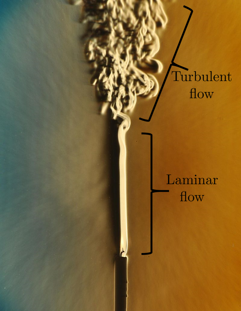
Fig. 14 This is a beautiful example of the difference between ordered and smooth laminar flow and chaotic turbulent flow.
A numeric way to determine whether flow is laminar or turbulent is by finding the Reynolds number, \({\rm Re}\). The Reynolds number is a dimensionless parameter that compares inertia, represented by the average flow velocity \(\bar v\) times a length scale \(D\) to viscosity, represented by the kinematic viscosity \(\nu\). Click here for a brief video explanation of viscosity. If the Reynolds number is less than 2,100 the flow is considered laminar. If it is more than 2,100, it is considered turbulent.
The transition between laminar and turbulent flow is not yet well understood, which is why the concept of transitional flow is often simplified and neglected to make it possible to code for laminar or turbulent flow, which are better understood. We will assume that the transition occurs at \(\rm{Re} = 2100\). In aguaclara, this parameter is pc.RE_TRANSITION_PIPE.
Fluid can flow through very many different geometries, like a pipe, a rectangular channel, or any other shape. To account for this, the characteristic length scale for the Reynolds number, which was written in the equation above as \(D\), is quantified as the hydraulic diameter, \(D_h\) when considering a general cross-sectional area. For circular pipes, which are the most common geometry you’ll encounter in this class, the hydraulic diameter is simply the pipe’s diameter, \(D_h = D\).
Here are other commonly used forms of the Reynolds number equation for circular pipes. They are the same as the one above, just with the substitutions \(Q = \bar v \frac{\pi D^2}{4}\) and \(\nu = \frac{\mu}{\rho}\)
See also
Function in aguaclara: pc.re_pipe(FlowRate, Diam, Nu) Returns the Reynolds number in a circular pipe. Functions for finding the Reynolds number through other flow conduits and geometries can also be found in physchem.py within aguaclara.
Note
Definition of Flow Regimes: Laminar and turbulent flow are described as two different flow regimes. When there is a characteristic of flow and different categories of the characteristic, each category is referred to as a flow regime. For example, the Reynolds number describes a flow characteristic, and its categories, referred to as flow regimes, are laminar or turbulent.
Streamlines and Control Volumes
Both streamlines and control volumes are tools to compare different parts of a system. For this class, this system will always be hydraulic.
Imagine water flowing through a pipe. A streamline is the path that a particle would take if it could be placed in the fluid without changing the original flow of the fluid. A more technical definition is “a line which is everywhere parallel to the local velocity vector.” Computational tools, dyes (in water), or smoke (in air) can be used to visualize streamlines.
A control volume is just an imaginary 3-dimensional shape in space. Its boundaries can be placed anywhere by the person applying the control volume, and once set the boundaries remain fixed in space over time. These boundaries are usually chosen to compare two relevant surfaces to each other. These surfaces are called Control Surfaces. The entirety of a control volume is usually not shown, as it is often unnecessary. This is demonstrated in the following image:
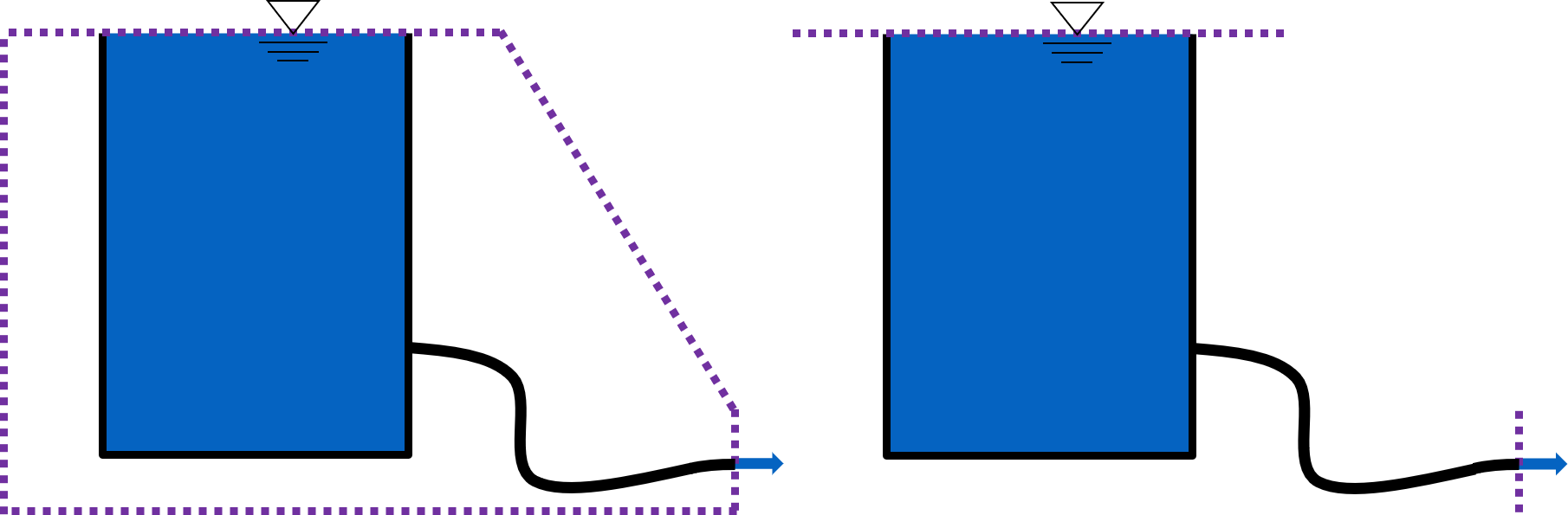
Fig. 15 While the image on the left indicates a complete control volume, control volumes are usually shortened to only include the relevant control surfaces, in which the control volume intersects the fluid. This is shown in the image on the right.
Important
Many images will be used over the course of this class to show hydraulic systems. A standardized system of lines will be used throughout them all to distinguish reference elevations from control volumes from streamlines. This system is described in the image below.
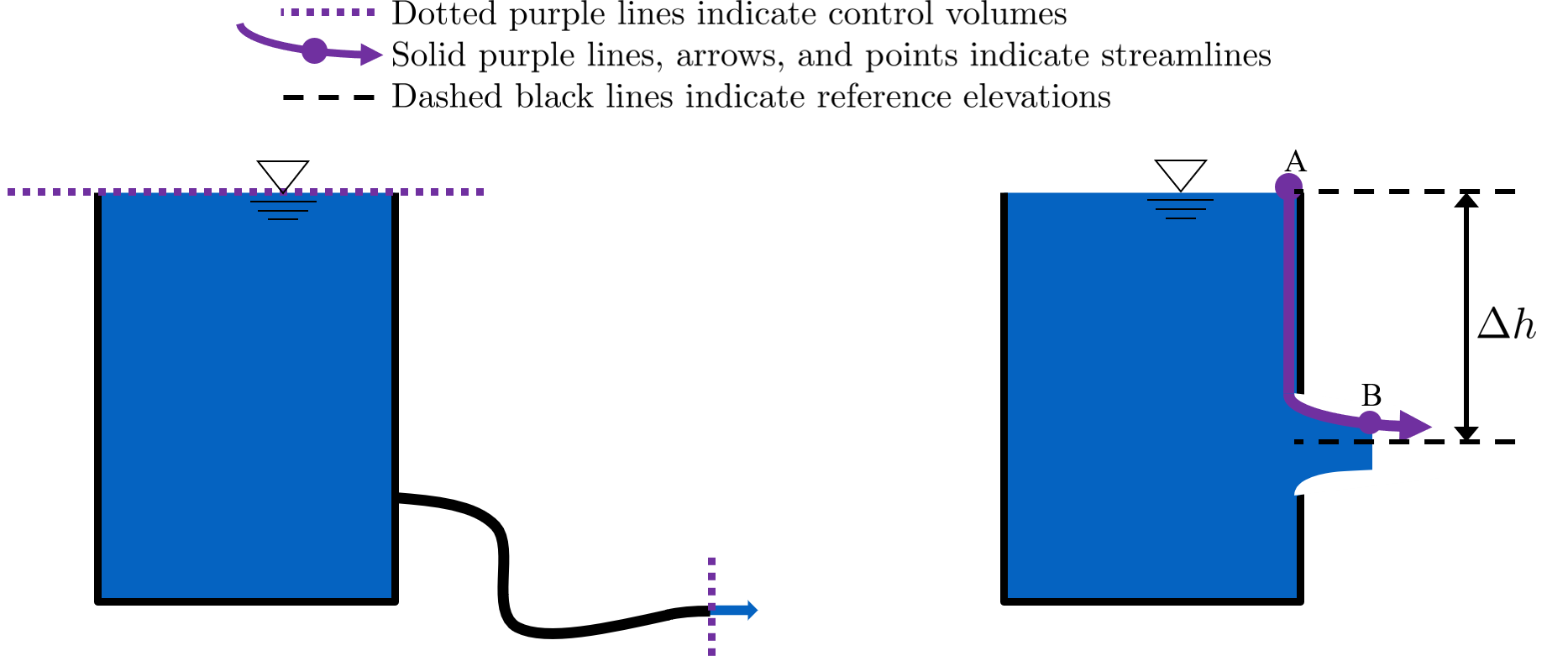
Fig. 16 On the left, a control volume is applied to a hydraulic system. On the right, a streamline is applied to a hydraulic system. A figure-convention for control volumes and streamlines will be very helpful throughout this course as there will be very, very many figures.
The Bernoulli and Energy Equations
As explained in almost every fluid mechanics class, the Bernoulli and energy equations are incredibly useful in understanding the transfer of the fluid’s energy throughout a streamline or through a control volume. The Bernoulli equation applies to two different points along one streamline, whereas the energy equation applies to fluid entering and exiting a control volume. The energy of a fluid has three forms: pressure, potential (deriving from elevation), and kinetic (deriving from velocity).
The Bernoulli Equation
These three forms of energy expressed above make up the Bernoulli equation:
Notice that each term in this form of the Bernoulli equation has units of \([L]\), even though the terms represent the energy of the fluid, which has units of \(\frac{[M] \cdot [L]^2}{[T]^2}\). When energy of the fluid is described in units of length, the term used is called head and referred to as \(h\).
There are two important distinctions to keep in mind when using head to talk about a fluid’s energy. First is that head is dependent on the density of the fluid under consideration. Take mercury, for example, which is around 13.6 times more dense than water. 1 meter of mercury head is therefore equivalent to around 13.6 meters of water head. Second is that head is independent of the amount of fluid being considered, as long as all the fluid is the same density. Thus, raising 1 liter of water up by one meter and raising 100 liters of water up by one meter are both equivalent to giving the water 1 meter of water head, even though it requires 100 times more energy to raise the hundred liters than to raise the single liter. Since we are concerned mainly with water in this class, we will refer to ‘water head’ simply as ‘head’.
Going back to the Bernoulli equation, the \(\frac{p}{\rho g}\) term is called the pressure head, \(z\) is called the elevation head, and \(\frac{v^2}{2g}\) is the velocity head. The following diagram shows these various forms of head via a 1 meter deep bucket (left) and a jet of water shooting out of the ground (right).
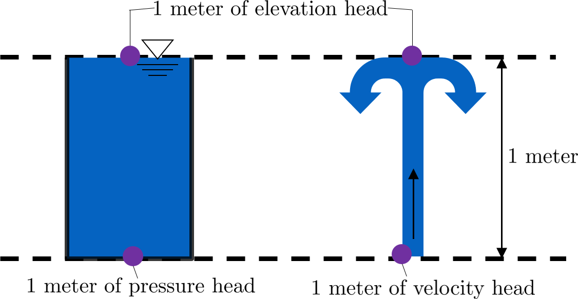
Fig. 17 The three forms of hydraulic head.
Though there are many assumptions needed to confirm that the Bernoulli equation can be used, the main one for the purpose of this class is that energy is not gained or lost throughout the streamline being considered. If we consider more precise fluid mechanics terminology, then “friction by viscous forces must be negligible.” What this means is that the fluid along the streamline being considered is not losing energy to viscosity. As a result, using the Bernoulli equation implies that energy can’t be gained or lost. It can only be transferred between its three forms.
Here is a simple worksheet with very straightforward example problems using the Bernoulli equation. Note that the solutions use the pressure-form of the Bernoulli equation. This just means that every term in the equation is multiplied by \(\rho g\), so the pressure term is just \(P\). The form of the equation does not affect the solution to the problem it helps solved.
The Control Volume Energy Equation
The assumption necessary to use the Bernoulli equation, which is stated above, represents the key difference between the Bernoulli equation and the control volume energy equation for the purpose of this class. The energy equation accounts for the potential addition or loss of fluid energy within the control volume. (L)oss of energy is usually due to viscous friction resisting fluid flow, \(h_L\), or the charging of a (T)urbine, \(h_T\). The most common input of fluid energy into a system is usually caused by a (P)ump within the control volume, \(h_P\).
You’ll also notice the \(\alpha\) term attached to the velocity head. This is a correction factor for kinetic energy, and will be neglected in this class; we assume that its value is 1. In the Bernoulli equation, the velocity of a streamline of the fluid is considered, \(v\). The energy equation, however compares control surfaces instead of streamlines, and the velocities across a control surface may not all be the same. Hence, \(\bar v\) is used to represent the average velocity. Since AguaClara does not use pumps nor turbines, \(h_P = h_T = 0\). With these simplifications, the energy equation can be written as follows:
This is the form of the energy equation that you will see over and over again in this book. To summarize, the main difference between the Bernoulli equation and the energy equation for the purposes of this class is energy loss. The energy equation accounts for the fluid’s loss of energy over time while the Bernoulli equation does not. So how can the fluid lose energy?
Head Loss
Head (L)oss, \(h_L\) is a term that is ubiquitous in both this class and fluid mechanics in general. Its definition is exactly as it sounds: it refers to the loss of energy of a fluid as it flows through space. There are two components to head loss: major losses caused by (f)riction between the fluid and the surface it’s flowing over, \(h_{\rm{f}}\), and minor losses caused by fluid-fluid internal friction resulting from flow (e)xpansions, \(h_e\). These two components combine such that \(h_L = h_{\rm{f}} + h_e\).
Major Losses
These losses are the result of friction between the fluid and the surface over which the fluid is flowing. A force acting parallel to a surface is referred to as shear. It can therefore be said that major losses are the result of shear between the fluid and the surface it’s flowing over. To help in understanding major losses, consider the following example: imagine, as you have so often in physics class, pushing a large box across the ground. Friction is what resists your efforts to push the box. The farther you push the box, the more energy you expend pushing against friction. The same is true for water moving through a pipe, where water is analogous to the box you want to move, the pipe is similar to the floor that provides the friction, and the major losses of the water through the pipe is analogous to the energy you expend by pushing the box.
In this class, we will be dealing primarily with major losses in circular pipes, as opposed to channels or pipes with other geometries. Fortunately for us, Henry Darcy and Julius Weisbach came up with a handy equation to determine the major losses in a circular pipe under both laminar and turbulent flow conditions. Their equation is logically and unoriginally named the Darcy-Weisbach equation. It is shown below:
Substituting the continuity Equation \(Q = \bar vA\) in the form of \(\bar v^2 = \frac{16Q^2}{\pi^2 D^4}\) gives another, equivalent form of Darcy-Weisbach which uses flow, \(Q\), instead of velocity, \(\bar v\):
See also
Function in aguaclara: pc.headloss_fric(FlowRate, Diam, Length, Nu, PipeRough) Returns only major losses. Works for both laminar and turbulent flow. PipeRough describes the pipe roughness \(\epsilon\) described shortly below.
Darcy-Weisbach is wonderful because it applies to both laminar and turbulent flow regimes and contains relatively easy to measure variables. The one exception is the Darcy friction factor, \(\rm{f}\). This parameter is an approximation for the magnitude of friction between the pipe walls and the fluid, and its value changes depending on the whether or not the flow is laminar or turbulent, and varies with the Reynolds number in both flow regimes.
For laminar flow, the friction factor can be determined from the following equation:
For turbulent flow, the friction factor is more difficult to determine. In this class, we will use the Swamee-Jain equation:
See also
Function in aguaclara: pc.fric(FlowRate, Diam, Nu, PipeRough) Returns \(\rm{f}\) for laminar or turbulent flow. For laminar flow, use zero for the PipeRough input.
The simplicity of the equation for \(\rm{f}\) during laminar flow allows for substitutions to create a very useful, simplified equation for major losses during laminar flow. This simplification combines the Darcy-Weisbach equation, the equation for the Darcy friction factor during laminar flow, and the Reynold’s number formula:
To form the Hagen-Poiseuille equation for major losses during laminar flow, and only during laminar flow:
The significance of this equation lies in its relationship between \(h_{\rm{f}}\) and \(Q\). Hagen-Poiseuille shows that the terms are directly proportional (\(h_{\rm{f}} \propto Q\)) during laminar flow, while Darcy-Weisbach shows that \(h_{\rm{f}}\) grows with the square of \(Q\) during turbulent flow (\(h_{\rm{f}} \propto Q^2\)). As you will soon see, minor losses, \(h_e\), will grow with the square of \(Q\) in both laminar and turbulent flow. This has implications that will be discussed in a future chapter: AguaClara Flow Control and Measurement Technologies.
In 1944, Lewis Ferry Moody plotted a ridiculous amount of experimental data, gathered by many people, on the Darcy-Weisbach friction factor to create what we now call the Moody diagram. This diagram makes it easy to find the friction factor \(f\). \(\rm{f}\) is plotted on the left-hand y-axis, relative pipe roughness \(\frac{\epsilon}{D}\) is on the right-hand y-axis, and Reynolds number \(\rm{Re}\) is on the x-axis. The Moody diagram is an alternative to computational methods for finding \(\rm{f}\).
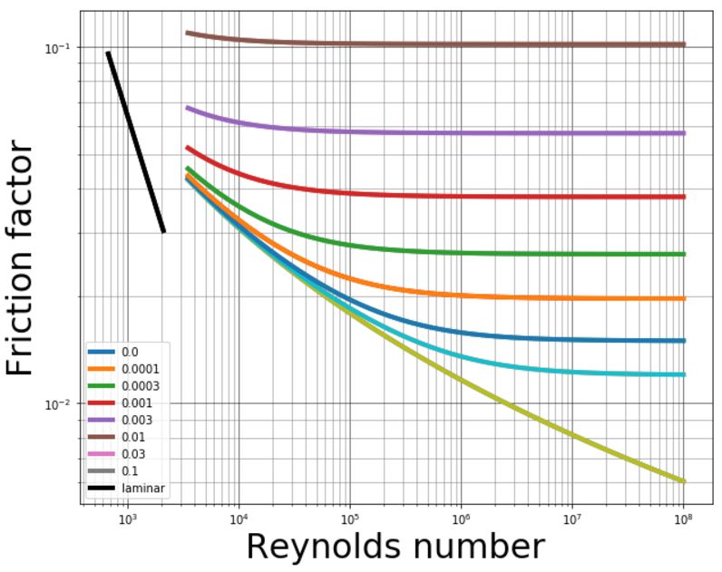
Fig. 18 This is the famous and famously useful Moody diagram.
Minor Losses
Unfortunately, there is no simple ‘pushing a box across the ground’ example to explain minor losses. So instead, consider a hydraulic jump. In the video, you can see lots of turbulence and eddies in the transition region between the fast, shallow flow and the slow, deep flow. The high amount of mixing of the water in the transition region of the hydraulic jump results in significant friction between water and water. This turbulent, eddy-induced, fluid-fluid friction results in minor losses, much like fluid-pipe friction results in major losses.
As occurs in a hydraulic jump, a flow expansion (from shallow flow to deep flow) creates the turbulent eddies that result in minor losses. This will be a recurring theme throughout the course: minor losses are caused by flow expansions. Imagine a pipe fitting that connects a small diameter pipe to a large diameter one, as shown in Fig. 19 below. The flow must expand to fill up the entire large diameter pipe. This expansion creates turbulent eddies near the union between the small and large pipes, and these eddies result in minor losses. You may already know the equation for minor losses, but understanding where it comes from is very important for effective AguaClara plant design. For this reason, you are strongly recommended to read through its full derivation: Fluid Mechanics Derivations.
The general form of the minor loss equation is
where \(\bar v\) is a characteristic (and perhaps convenient) velocity that is typically based on the flow rate and the dimensions of the fully expanded flow. Thus minor loss coefficients, \(K_e\) for flow through various pipe fittings are based on the average velocity in the pipe because that is easily known given the pipe internal diameter and the flow rate.
There are three forms of the minor loss equation that you will see in this class:
Note
You will most often see \(K_e^{'}\) and \(K_e\) used without the \(e\) subscript, as \(K^{'}\) and \(K\).
See also
Function in aguaclara: pc.headloss_exp_general(Vel, KMinor) Returns \(h_e\). Can be either the second or third form due to user input of both velocity and minor loss coefficient. It is up to the user to use consistent \(\bar v\) and \(K_e\).
See also
Function in aguaclara: pc.headloss_exp(FlowRate, Diam, KMinor) Returns \(h_e\). Uses third form, \(K_e\).
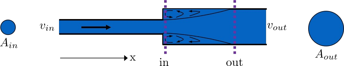
Fig. 19 The \(in\) and \(out\) subscripts in each of the three forms of the minor loss equation refer to this diagram that was used for the derivation.
The second and third forms are the ones which you are probably most familiar with. The distinction between them, however, is critical. First, consider the magnitudes of \(A_{in}\) and \(A_{out}\). \(A_{in}\) can never be larger than \(A_{out}\), because the flow is expanding. When flow expands, the cross-sectional area it flows through must increase. As a result, both \(\frac{A_{out}}{A_{in}} > 1\) and \(\frac{A_{in}}{A_{out}} < 1\) must always be true. This means that \(K^{'}\) can never be greater than 1, while \(K\) technically has no upper limit.
If you have taken CEE 3310, you have seen tables of minor loss coefficients like this one, and they almost all have coefficients greater than 1. This implies that these tables use the third form of the minor loss equation as we have defined it, where the velocity is \(\bar v_{out}\). There is a good reason for using the third form over the second one: \(\bar v_{out}\) is far easier to determine than \(\bar v_{in}\). Consider flow through a pipe elbow, as shown in the image below.
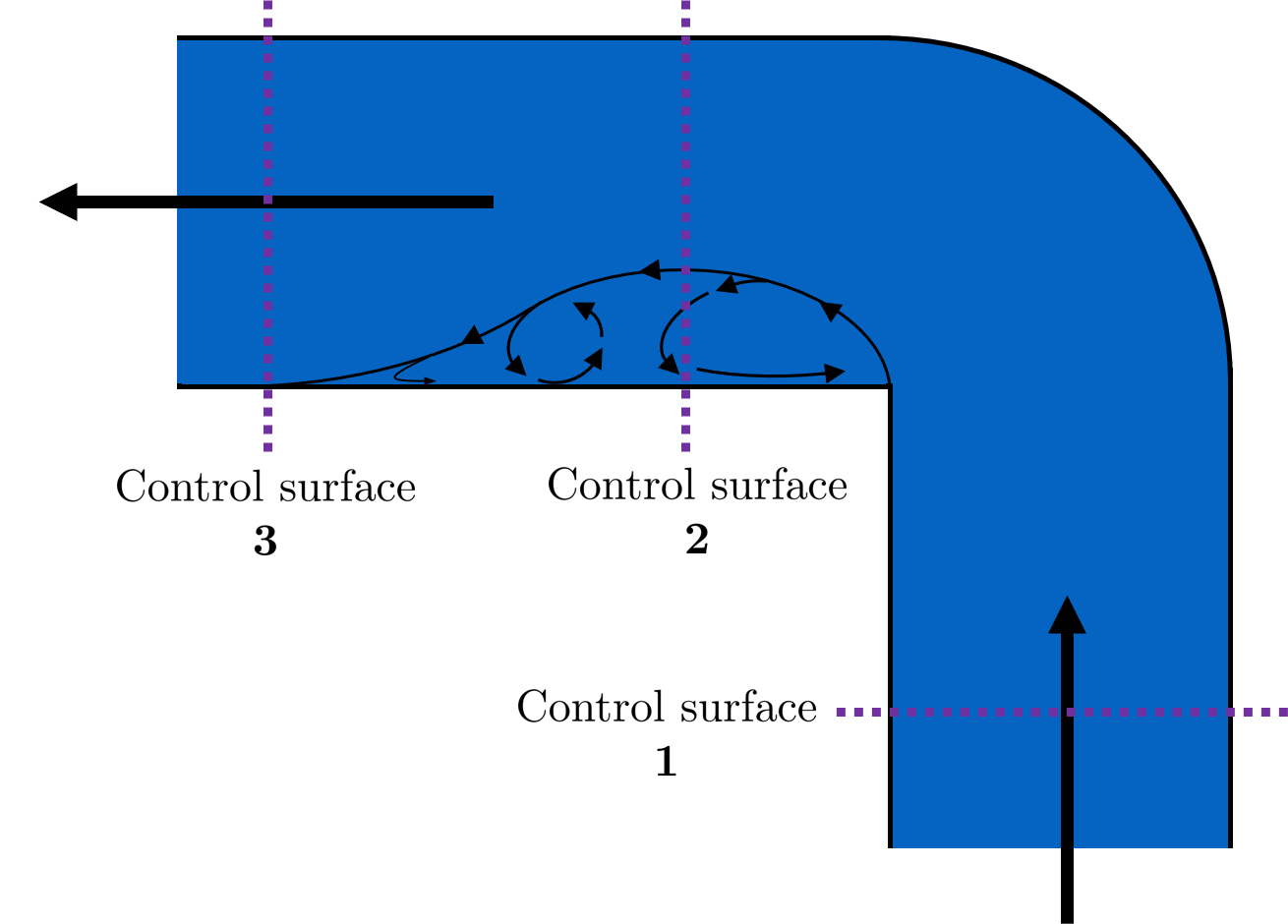
Fig. 20 Flow around a pipe elbow results in a minor loss. ‘Control surface 1’ can be abbreviated as ‘CS 1’
In order to find \(\bar v_{out}\), we first need to know what (or where) is \(out\) and what is \(in\). A simple way to distinguish the two surfaces is that \(in\) occurs when the flow is most contracted, and \(out\) occurs when the flow has fully expanded after that maximal contraction. Going on these guidelines, Control surface ‘2’ (CS 2) in the figure above would be \(in\), since it represents the most contracted flow in the elbow-pipe system. Therefore, CS 3 would be \(out\), as it represents the flow having fully expanded after its compression at CS 2.
\(\bar v_{out}\) is easy to determine because it is the velocity of the fluid as it flows through the entire area of the pipe. Thus, \(\bar v_{out}\) can be found with the continuity equation, since the flow through the pipe and its diameter are easy to measure, \(\bar v_{out} = \frac{4 Q}{\pi D^2}\). On the other hand, \(\bar v_{in}\) is difficult to find, as the area of the contracted flow is dependent on the exact geometry of the elbow. This is why the third form of the minor loss equation, as we have defined it, is the most common:
Note
When considering a hydraulic system within a control volume, there can be many sources of minor losses. Instead of saying \(h_e = K_1 \frac{\bar v_{out}^2}{2g} + K_2 \frac{\bar v_{out}^2}{2g} + ...\) we can simply lump all of the minor loss coefficients into one: \(\sum K = K_1 + K_2 + ...\). Thus, it is also common to see this form of the minor loss equation when finding the minor loss across control volumes: \(\sum K \frac{v_{out}^2}{2g}\).
The Head Loss Elevation Trick
This trick, also called the ‘control volume trick,’ or more colloquially, the ‘head loss trick,’ is incredibly useful for simplifying hydraulic systems and is used all the time in this class.
Consider the following figure:
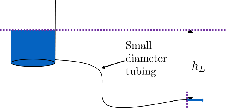
Fig. 21 A typical hydraulic system can be used to understand the head loss trick.
In systems like this, where an elevation difference is causing water to flow, the elevation difference is called the driving head. In the system above, the driving head is the elevation difference between the water level and the end of the tubing. Usually, driving head is written as \(\Delta z\) or \(\Delta h\), though above it is labelled as \(h_L\). Doesn’t \(h_L\) refer to head loss though? Yes it does! Referring to \(\Delta h\) or \(\Delta z\) IS the head loss trick, and how it works is explained in the following paragraphs and equations.
The figure is technically violating the energy equation by saying that the elevation difference between the water in the tank and the end of the tube is \(h_L\). It implies that all of the driving head, \(\Delta z\), is lost to head loss. Since all of the energy is gone, there should not be water flowing out of the tubing. But there is. Let’s apply the energy equation across the control surfaces shown in the figure. Pressures at both ends are atmospheric and the velocity of water at the top of tank is negligible.
We now get:
This equation contradicts the figure above, which says that \(\Delta z = h_L\) and neglects \(\frac{\bar v_2^2}{2g}\). The figure above is correct, however, if you apply the head loss trick. The trick incorporates the \(\frac{\bar v_2^2}{2g}\) term into the \(h_L\) term as a minor loss. See the math below:
This last step incorporated the kinetic energy term of the energy equation, \(\frac{\bar v_2^2}{2g}\), into the minor loss equation by saying that its \(K\) is 1 and incorporating that 1 into \(\sum K\). From here, we reverse our steps to get \(\Delta z = h_L\), starting with \(h_e = \left( \sum K \right) \frac{\bar v_2^2}{2g}\)
By applying the head loss trick, you are considering the entire flow of the fluid out of a control volume as energy lost via minor losses. This is just an algebraic trick, the only thing to remember when applying this trick is that \(\sum K\) will always be at least 1, even if there are no ‘real’ minor losses in the system.
Vena Contracta and The Orifice Equation
This equation is one that you’ll see and use again and again throughout this class. Understanding it now will be invaluable, as future concepts will use and build on this equation.
Vena Contracta
Before describing the equation, we must first understand the concept of a vena contracta. Refer to the figure below.
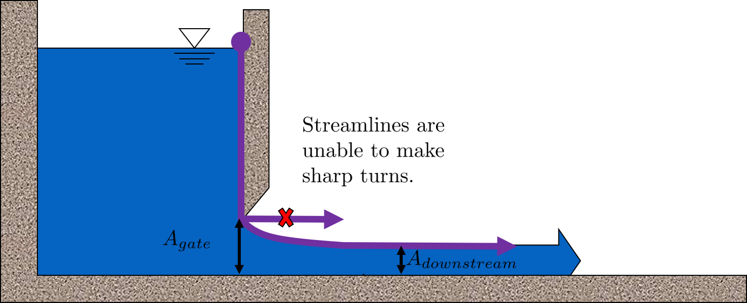
Fig. 22 This figure shows flow around a sluice gate. Since streamlines can’t make sharp turns, the flow is forced to gradually curve and contract to an area smaller than the area of the gate.
The flow contracts as the fluid moves past the gate. This happens because the fluid can’t make a sharp turn as it tries to go around the gate, as indicated by the streamline in the figure. Instead, the most extreme streamline makes a gradual change in direction. As a result of this gradual turn, the flow contracts and the cross-sectional area the fluid is flowing decreases.
The term ‘vena contracta’ describes the phenomenon of contracting flow due to streamlines being unable to make sharp turns. \(\Pi_{vc}\) is a dimensionless ratio comparing the flow area at the point of maximal contraction, \(A_{downstream}\), and the flow area before the contraction, \(A_{gate}\). In the figure above, the equation for the vena contracta coefficient would be:
The vena contracta for an infinite slot such as the sluice gate in Fig. 22 has an analytical solution (see McDonald, 2005: Vena Contracta) given by
where Equation (13) assumes the most extreme turn a streamline must make is \(\frac{\pi}{2}\). This parameter value, 0.611, is in aguaclara python library as pc.VC_ORIFICE_RATIO. The vena contracta coefficient value is a function of the flow geometry and specifically the most extreme turn a streamline takes. Equation (13) can be generalized to any streamline angle, \(\theta\), with the assumption that we need a function that returns 1 for an angle of 0 and for an angle of \(\pi\) it must return \(\left(\Pi_{vc_{\frac{\pi}{2}}}\right)^2\).
Equation (14) will be useful when we evaluate flocculator baffles that have an angle of \(\pi\) as the water flows around the end of a baffle.
Important
A vena contracta coefficient is not a minor loss coefficient. Though the equations for the two both involve contracted and non-contracted areas, these coefficients are not the same. Minor losses coefficients imply energy loss, and vena contractas do not. Minor losses coefficients deal with flow expansions, and vena contractas deal with flow contractions. Confusing the two coefficients is common mistake that this paragraph will hopefully help you to avoid.
Note
Note that \(\Pi_{vc}\) is often referred to as a ‘Coefficient of Contraction,’ \(C_c\), in other engineering courses and textbooks.
The Orifice Equation
The orifice equation is derived from the Bernoulli equation as applied to the purple points in the following image:
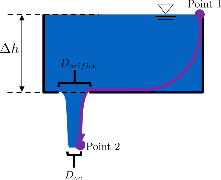
Fig. 23 Flow through a hole in the bottom of a bucket is a great example of the orifice equation.
At point 1, the pressure is atmospheric and the instantaneous velocity is negligible as the water level in the bucket drops slowly. At point 2, the pressure is also atmospheric. We define the difference in elevations between the two points, \(z_1 - z_2\), to be \(\Delta h\). With these simplifications \((p_1 = \bar v_1 = p_2 = 0)\) and assumptions \((z_A - z_B = \Delta h)\), the Bernoulli equation becomes:
Substituting the continuity Equation \(Q = \bar v A\) in the form of \(\bar v_2^2 = \frac{Q^2}{A_{vc}^2}\), the vena contracta coefficient in the form of \(A_{vc} = \Pi_{vc} A_{or}\) yields:
Which, rearranged to solve for \(Q\) gives The Orifice Equation:
pc.VC_ORIFICE_RATIOSee also
Equation in aguaclara: pc.flow_orifice(Diam, Height, RatioVCOrifice) Returns flow through a horizontal orifice.
See also
Equation in aguaclara: pc.flow_orifice_vert(Diam, Height, RatioVCOrifice) Returns flow through a vertical orifice. The height parameter refers to height above the center of the orifice.
There are two configurations for an orifice in the tank holding a fluid: horizontal and vertical. These are both displayed in the figure below. The orifice equation written is for a horizontal orifice; the equation for flow through a vertical orifice equation requires integration or the orifice equation across its height to return the correct flow. This is explored in the Flow Control and Measurement Examples section.
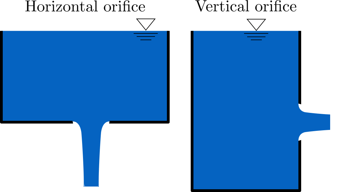
Fig. 24 The descriptions ‘vertical’ and ‘horizontal’ apply to the orientation of the orifices, not to the orientation of the fluid coming out of the orifices.
Section Summary
Introductory Concepts:
Continuity means that the mass of a fluid is conserved as it flows, and implies a constant density. The continuity equation has two purposes:
Relating the average velocity of a fluid, \(\bar v\), to its flow rate, \(Q\), via the cross-sectional area, \(A\), that it flows through. When the fluid is flowing in a pipe, we can simply expand this even further to relate the flow rate and velocity to the pipe’s diameter, \(D\). The final equation below is only used for circular pipes, as it includes a pipe diameter.
\[Q = \bar v A = \bar v \frac{\pi D^2}{4}\]Finding the average velocity or flow when the geometry of a fluid’s flow changes, as the mass of the fluid must be conserved when it transitions through flow geometries.
\[Q_1 = Q_2\]\[\bar v_1 A_1 = \bar v_2 A_2\]\[\bar v_1 \frac{\pi D_1^2}{4} = \bar v_2 \frac{\pi D_2^2}{4}\]Laminar and Turbulent flow describe the disorder and chaos of fluid flow. The Reynolds number, \({\rm Re}\) is used to distinguish laminar from turbulent flow. For \({\rm Re} < 2100\), flow is considered laminar. For \({\rm Re} > 2100\), flow is considered turbulent. The equations for the Reynolds number are below:
\[{\rm Re} = \frac{\bar vD}{\nu} = \frac{4Q}{\pi D\nu} = \frac{\rho \bar vD}{\mu}\]Control volumes vs Streamlines. This section is quite short, a summary would simply repeat what the section says. The section is its own summary; read it here: Streamlines and Control Volumes
Bernoulli vs Energy equations: The Bernoulli equation assumes that energy is conserved throughout a streamline or control volume. The Energy equation assumes that there is energy loss, or head loss \(h_L\). This head loss is composed of major losses, \(h_{\rm{f}}\), and minor losses, \(h_e\).
Bernoulli equation:
\[\frac{p_1}{\rho g} + {z_1} + \frac{\bar v_1^2}{2g} = \frac{p_2}{\rho g} + {z_2} + \frac{\bar v_2^2}{2g}\]Energy equation, simplified to remove pumps, turbines, and \(\alpha\) factors:
\[\]frac{p_{1}}{rho g} + z_{1} + frac{bar v_{1}^2}{2g} = frac{p_{2}}{rho g} + z_{2} + frac{bar v_{2}^2}{2g} + h_L
Major losses: Defined as the energy loss due to shear between the walls of the pipe/flow conduit and the fluid. The Darcy-Weisbach equation is used to find major losses in both laminar and turbulent flow regimes. The equation for finding the Darcy friction factor, \(\rm{f}\), changes depending on whether the flow is laminar or turbulent. The Moody diagram is a common graphical method for finding \(\rm{f}\). During laminar flow, the Hagen-Poiseuille equation, which is just a combination of Darcy-Weisbach, Reynolds number, and \({\rm{f}} = \frac{64}{\rm{Re}}\), can be used
Darcy-Weisbach equation:
\[h_{\rm{f}} = {\rm{f}} \frac{L}{D} \frac{\bar v^2}{2g}\]For water treatment plant design we tend to use plant flow rate, \(Q\), as our master variable and thus we have.
\[h_{\rm{f}} = {\rm{f}} \frac{8}{g \pi^2} \frac{LQ^2}{D^5}\]\(\rm{f}\) for laminar flow:
\[{\rm{f}} = \frac{64}{\rm{Re}} = \frac{16 \pi D \nu}{Q} = \frac{64 \nu}{\bar v D}\]\(\rm{f}\) for turbulent flow:
\[{\rm{f}} = \frac{0.25} {\left[ \log \left( \frac{\epsilon }{3.7D} + \frac{5.74}{{\rm Re}^{0.9}} \right) \right]^2}\]Hagen-Poiseuille equation for laminar flow:
\[h_{\rm{f}} = \frac{32\mu L \bar v}{\rho gD^2} = \frac{128\mu Q}{\rho g\pi D^4}\]
Minor losses: Defined as the energy loss due to the generation of turbulent eddies when flow expands. Once more: minor losses are caused by flow expansions. There are three forms of the minor loss equation, two of which look the same but use different coefficients (\(K^{'}\) vs \(K\)) and velocities (\(\bar v_{in}\) vs \(\bar v_{out}\)). Make sure the coefficient you select is consistent with the velocity you use. The third form, written in purple, is the most commonly used form of the minor loss equation.
Major and minor losses vary with flow: While it is generally important to know how increasing or decreasing flow will affect head loss, it is even more important for this class to understand exactly how flow will affect head loss. As the table below shows, head loss will always be proportional to flow squared during turbulent flow. During laminar flow, however, the exponent on \(Q\) will be between 1 and 2 depending on the proportion of major to minor losses.
\(h_L propto Q^?\) |
Major Losses |
Minor Losses |
|---|---|---|
Laminar |
\(Q\) |
\(Q^2\) |
Turbulent |
\(Q^2\) |
\(Q^2\) |
The head loss trick, also called the control volume trick, can be used to incorporate the ‘kinetic energy out’ term of the energy equation, \(\frac{\bar v_2^2}{2g}\), into head loss as a minor loss with \(K = 1\), so the minor loss equation becomes \(\left( 1 + \sum K \right) \frac{\bar v^2}{2g}\). This is used to be able to say that \(\Delta z = h_L\) and makes many equation simplifications possible in the future.
Orifice equation and vena contractas: The orifice equation is used to determine the flow out of an orifice given the elevation of water above the orifice. This equation introduces the concept of vena contracta, which describes flow contraction due to the inability of streamlines to make sharp turns. The equation shows that the flow out of an orifice is proportional to the square root of the driving head, \(Q \propto \sqrt{\Delta h}\). Depending on the orientation of the orifice, vertical (like a hole in the side of a bucket) or horizontal (like a hole in the bottom of a bucket), a different equation in AguaClara should be used.
The Orifice Equation:
\[Q = \Pi_{vc} A_{or} \sqrt{2g\Delta h}\]