Coagulant Automation
Automating the coagulant dose is difficult because it hasn’t been clear what measurement to use that could be driven to a target value by varying the coagulant dose and that would then provide the desired plant performance. Based on the previous understanding of coagulant neutralizing the negative charge of raw water particles, many water treatment plants have attempted to use streaming current meters to set the coagulant dose. That method doesn’t work well because it is the fractional coverage of the primary particles with sticky coagulant nanoparticles that sets the attachment efficiency and that does not require a neutral surface charge.
The concentration of primary particles exiting the flocculator could be used to guide the coagulant dose. The flocculated suspension can not be sampled directly with a particle counter because the particle concentration is too high. Given that we are only interested in the concentration of primary particles, we can use a tube settler to quickly reduce the particle concentration of the sample line going to the particle counter while still enabling an accurate count of the primary particle concentration.
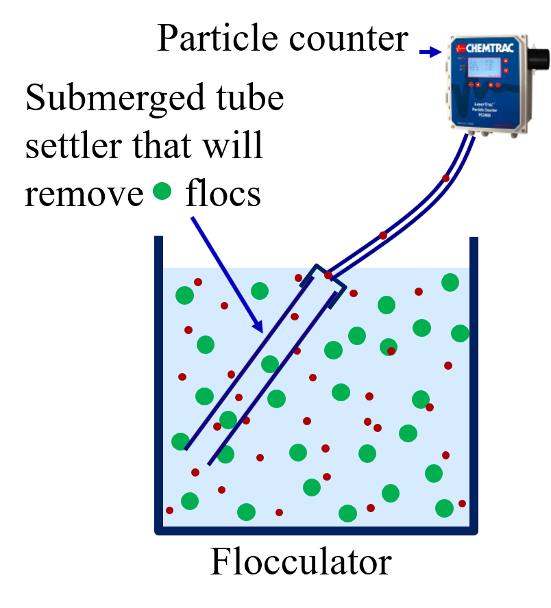
Fig. 240 Proposed particle counter monitoring of flocculation performance.
Coagulant Dose for Suspended Particles
The relationship between attachment efficiency and primary particle concentration after flocculation is given by Equation (180). For the simple case of no coagulant demand by dissolved organic matter it is reasonable to assume that the attachment efficiency is proportional to the ratio of the coagulant dose to the surface area of the particles in the raw water and the particle surface area is proportional to the particle concentration.
This coagulant dose only refers to the coagulant that will end up coating the suspended particles. The coagulant nanoparticles that are coated by dissolved organic matter will be considered in the next section.
The result of the AguaClara flocculation model (Equation (177)) is repeated here for convenience.
Substituting Equation (372) and solving for the coagulant dose we obtain
The primary particle properties and flocculator design terms can be treated as a single unknown, \(k_{pf}\).
Thus Equation (374) simplifies to
Coagulant Dose for Dissolved Organic Matter
The next improvement in this simple model is to add a correction factor for dissolved organic matter. The dissolved organic matter effectively inactivates some of the coagulant. The dissolved organic matter is measured as absorbance at 254 nm. The amount of coagulant that is tied up with dissolved organic matter is
The dissolved organic matter simply reduces the amount of coagulant that is available to make the inorganic particles sticky. The required coagulant dose can be obtained by adding \(C_{coag_{DOM}}\) to Equation (376).
One method to estimate \(K_{DOM}\) is based on the experimental results obtained by Yingda Du (see Fig. 125 by Yingda Du, et al., 2019). Those results suggest that approximately 1 mg/L of aluminum is required to tie up 12 mg/L of humic acid. The humic acid concentration was based on the dry weight and humic acid is approximately 48% carbon. Thus 6 mg of humic acid as carbon require 1 mg/L of aluminum. The absorbance at 254 nm was measured by Rodrigues. et al., 2008 to be 0.055(humic acid as carbon in mg/L). Thus \(0.33A_{254nm}\) is expected to consume 1 mg/L of aluminum where \(A_{254nm}\) is the UV 254 absorbance in a 1 cm sample cell. The remaining required conversion is from the concentration of aluminum to the coagulant dose as measured at the water treatment plant.
Equation (378) can be rewritten with subscripts that indicate when and where the samples are taken for the application of automatic coagulant dosing. The tube settler turbidity in the future, \(C_{TS_{flocculated_{t + \theta}}}\) is the target turbidity of flocculated water after passing through a tube settler that we are trying to obtain.
Equation (379) reveals that there is an important time lag due to the hydraulic retention time between the coagulant injection and the clarified water sample. This time lag will require that the dosing algorithm include data from the recent history to account for this time offset.
Simple Corrector Method
An estimate for the coagulant demand of the DOM is obtained by solving Equation (379) for \(C_{coag_{DOM_{t}}}\) and shifting the time to one hydraulic residence time earlier.
Given the estimate of the DOM coagulant demand a hydraulic residence time earlier we can obtain an estimate of the current required coagulant dose. We will use Equation (379) and the assumption that the coagulant DOM demand doesn’t change significantly in one hydraulic residence time. The \(C_{TS_{flocculated_{t + \theta}}\) is the target tube settler turbidity.
The coagulant dosing system must include guardrails to ensure that the coagulant dose is within a reasonable range. The potential failures include:
incorrect reading from a turbidimeter due to an air bubble, a dirty sample cell, or during routine maintenance
settled water turbidity that is very low because the plant is starting up after an extended shutdown
Another potential failure mode would occur if the raw water turbidity is lower than the target clarified turbidity. This would result in a coagulant dose that could be too low to achieve effective filtration.
To reduce the likelihood of a treatment failure the estimated DOM coagulant demand can be compared with a reasonable range and if it is out of that range the estimated DOM coagulant demand can be forced back into the reasonable range. To prevent an excessively low coagulant dose the DOM coagulant demand can be limited to positive values. If it is known that the DOM coagulant demand is always exceeds a larger value, that larger value can be used as a lower limit. The upper limit can be set based on observation of the raw water quality.
Data processing
Acquire data at some high rate (perhaps 1 s intervals)
Set the number of coagulant dose updates per hydraulic residence time (HRT) (perhaps 10) and average the incoming data to that update interval
Hold the averaged data in a buffer with each data set including a time stamp.
For each coagulant dose update use Equation (380) to estimate the coagulant demand of the DOM and then use Equation (381) to estimate the new coagulant dose.
Floc Filtration Modification
We hypothesize that there is significant particle removal by floc filtration both in conventional sedimentation tanks and in the floc filter of the AguaClara clarifier. This means that the \(C_{TS_{flocculated_{t + \theta}}}\) is not a constant value, since it needs to account for the removal efficiency of the floc filter. Equation (382) calculates the total removal based on performance
where it is understood that these water samples are all passed through a tube settler, TS, before measuring the particle concentration.
Instead of setting a target for \(C_{TS_{flocculated}}\) we will set a target for \(C_{TS_{flocFiltered}}\). Equation (251) describes particle removal by settling flocs. The Equation (162) gives the relationship between floc concentration and its surrounding volume.
The \(\forall_{\rm{Surround}}\) is for the flocs that will be falling through the suspension. Thus it does not include the particles that are too small to settle significantly. The surrounding volume for the flocs in the sedimentation tank \(\forall_{\rm{Surround}}\) is a function of the floc concentration, \(\left( C_{raw} - C_{TS_{flocculated}} \right)\). From Equation (383) we have
The volume cleared can also be thought of as inversely proportional to a high turbidity where the \(\forall_{\rm{Surround}}\) is equal to the \(\forall_{\rm{Cleared}}\). We designate this concentration or turbidity as \(C_{Cleared}\).
Combining Equations (384) and (385) we obtain
Now we can simplify Equation (251) by substituting in Equation (386).
A possible solution method is to use a running approximation for the exponential term based on the previous measurement of \(C_{TS_{flocculated}}\).
The value of \(C_{TS_{flocFiltered_{t + \theta}}}\) is the target performance for the water leaving the conventional sedimentation tank. At each time step first use Equation (388) to obtain an estimate of the target for the turbidity after flocculation and a tube settler, \(C_{TS_{flocculated_{t + \theta}}}\). The result from Equation (388) can then be substituted into Equation (381) to calculate the new coagulant dose.
Still need to figure out the correction method for Need to think carefully about the time for measurement of each of these parameters and the various \(\theta\) involved.
Unfortunately this can’t be solved for \(C_{TS_{flocculated}}\), but we can solve for the settled water turbidity, \(C_{TS_{flocFiltered}}\). We invert the fraction and put a negative sign in the exponent.