Flocculation Derivations
Baffle Minor Loss Coefficient
For contractions in series the minor loss coefficient is strongly influenced by the distance between the contractions. When the contractions are spaced so closely that the flow can’t fully expand between contractions the velocity exiting the contraction is greater and the resulting head loss is greater. The distance required for the flow to expand can be estimated based on jet expansion equations. The flow exiting a rectangular contraction can be modeled as a plane jet and plane jets grow in width at a rate
where x is the distance along the path of the jet centerline and \(\Pi_{PlaneJet_{exp}} = 0.116\) for a plane jet in an infinite medium. The location of this expanding jet is shown in Figure Fig. 127. The jet is influenced by the presence of the baffle on the one side. Andrew Pennock, 2022, used Computational Fluid Dynamics (CFD) to determine that the jet is effectively only expanding on the side that is in contact with the recirculation zone. Thus
where \(\Pi_{BaffleJet_{exp}}\) is the dimensionless rate of expansion for the jet that has a baffle on the one side.
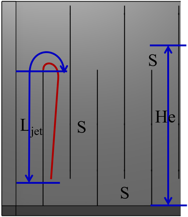
Fig. 127 Baffle geometry for a hydraulic flocculator where S is the space between baffles, \(L_{jet}\) is the distance over which a jet can expand, and \(H_e\) is the approximate total distance between expansions.
The distance over which the jet can expand is given by \(L_{jet}\). The path length is given by
where \(L_{curve}\) is the effective length of the curved path of the jet around the end of the baffle.
There may be an additional complication in assessing the jet path length. The jet continues to expand through the flow contraction and a dimensionless path length created by dividing the path length by the local jet width may makes the curved path at the end of the baffle even more significant.
The maximum width of the expanding jet, \(W_{jet_{max}}\), occurs immediately upstream of where the streamlines begin to curve to go around the end of the baffle. The jet minimum width (greatest contraction) occurs shortly after going around the 180° bend. Given that the flow might not have fully expanded we can express the jet minimum width as a function of the jet maximum width.
where \(\Pi_{vc}^{baffle}\) is given by Equation (14) with an angle of \(\pi\) and has a value of 0.3733. The maximum jet width is determined by how much it can expand in distance \(L_{jet}\).
Equations (189) and (190) provide two equations in two unknowns. Eliminate \(W_{jet_{min}}\) from Equation (190).
The velocity in the expanded jet is higher than would have been obtained based on continuity and the dimensions of the flow passage. The effect of the higher velocity can be factored into Equation (166) by multiplying by the ratio of the velocity squared. From continuity the ratio of \(S\) to \(W_{jet_{max}}\) is the ratio of the velocity in the expanded jet to the velocity that would have occurred if the flow had filled the enter flow passage. Substitute Equation (191) to obtain
The ratio of \(\frac{L_{jet}}{S}\) can be expressed as a function of the baffle ratio, \(\Pi_{H_eS}\). The maximum path length for jet expansion is used here.
Substitute Equation (193) into Equation (192) to obtain the ratio of the velocity in the expanded jet to the velocity that would have occurred if the flow had filled the enter flow passage.
Equation (194) has a minimum value of 1 representing fully expanded flow. For large values of \(\Pi_{H_eS}\) the equation would incorrectly predict values less than 1. This length ratio is also a velocity ratio given continuity and can be factored into the baffle minor loss equation (Equation (166)) to handle baffles in series where the flow doesn’t fully expand between baffles.
Equation (195) can be simplified to obtain
Equation (196) incorporates two assumptions that need to be checked with computational fluid dynamics.
The \(\Pi_{BaffleJet_{exp}}\) may be missing a correction to account for a secondary effect of the baffle.
The effective dimensionless length of the curved and contracted flow path, \(\Pi _{LS_{curve}}'\), is unknown.
Andrew Pennock conducted CFD analysis (see Fig. 128) to estimate the baffle loss coefficient as a function of the \(\Pi_{H_{e}S}\) (see Fig. 129) and used error minimization to estimate the previous two factors. The baffle jet expansion rate had a value of approximately \(0.5 \Pi_{PlaneJet_{exp}}\). This result is consistent with the idea that the jet is expanding into the zone of recirculation and is not expanding on the side of the jet that is against the baffle.
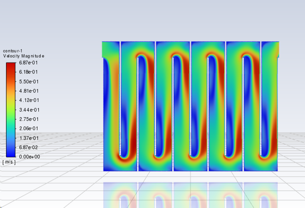
Fig. 128 CFD analysis of flow around baffles with \(\Pi_{H_{e}S} = 8\) showing the gradual flow expansion and return to a nearly uniform velocity before making the next bend (Andrew Pennock, 2022).
If we take \(\Pi_{BaffleJet_{exp}} = 0.5 \Pi_{PlaneJet_{exp}}\) as a given, then the remaining unknown is the dimensionless length of the curved and contracted flow path, \(\Pi _{LS_{curve}}'\). Andrew Pennock found \(\Pi _{LS_{curve}}' = 4.3\) using CFD. We also obtained one head loss measurement from the Gracias AguaClara plant shortly after the plant was first commissioned. It became apparent that the flocculator head loss exceeded the expected values because water was overflowing at the upstream end of the flocculator. The calculated \(K_{baffle_{exp}}\) for the original design of the Gracias flocculator is plotted in Fig. 129. The model fit through that single data point requires the dimensionless distance for the jet to fully expand to be \(\Pi _{LS_{curve}}' = 3\).
Given the slight disagreement between the two sources of information, CFD and a single head loss measurement at the Gracias AguaClara plant, it isn’t clear which value to use for \(\Pi _{LS_{curve}}'\). Further research is required and hydraulic flume experiments could provide the most definitive answer.
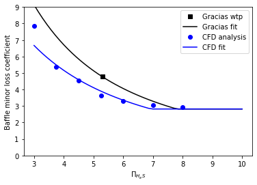
Fig. 129 Baffle minor loss coefficient (Equation (196)) was fit to the CFD analysis by Andrew Pennock. Additional data is needed to resolve the difference between the CFD analysis and the data point from the Gracias AguaClara plant.
Until further results are obtained we need to make an engineering judgement to select the least risky model for the baffle loss coefficient. Given a fully fabricated flocculator it is easier to reduce the baffle spacing by shortening the spacers between baffles than it is to increase the baffle spacing. Thus it would be best to err on the side of obtaining less head loss than the design specifications. To obtain less head loss than predicted we need to use the maximum estimate of \(K_{baffle_{exp}}\). The Gracias measurement gives the maximum estimate of \(K_{baffle_{exp}}\) based on \(\Pi _{LS_{curve}}' = 3\).
Equation (196) may need to be modified when we have more experimental or CFD results to provide a better estimate of the baffle loss coefficient.
The insight that the jet expands at half the rate of a free jet means that the jet doesn’t fully expand as quickly as we had thought prior to 2022. It isn’t until a \(\Pi_{H_eS}\) of about 8 that the jet is fully expanded and thus it is very reasonable to use \(\Pi_{H_eS}\) of 8 for design.
Linking head loss, velocity gradient, and geometry
The energy dissipation rate in Equation (46) can be set equal to the energy dissipated in a control volume given by Equation (52) to obtain
Equation (197) can be applied to a control volume that contains an entire flocculator or to a control volume containing a single flow expansion. Here we develop the analysis of a single flow expansion. This means that the residence time is the time between expansions, \(\theta_e\), and the head loss is for one expansion, \(h_{L_{e}}\).
From here we make three subsequent substitutions: first \(h_{L_{e}} = K_{baffle} \frac{\bar v^2}{2g}\), then \(\theta_e = \frac{H_e}{\bar v}\), and finally \(\bar v = \frac{Q}{WS}\).
where \(S\) is the distance between baffles, \(W\) is the dimension of the flow that is normal to \(S\) and \(H_e\) the distance between expansions. For complex geometry the best way to estimate \(H_e\) is the volume of water divided by \(WS\).
Equation (198) describes the relationship between the geometry of the flocculator, the flow rate, and the resulting velocity gradient.
Channel or Flow Width
The minimum allowable width of a Horizontal-Vertical flocculator channel is based on the requirements that \(\Pi_{H_eS_{min}} < \Pi_{H_eS} < \Pi_{H_eS_{max}}\) and that we maintain the \(\tilde{G}\) that serves as a basis for design. The final parameter derived is \(W_{min, \, \Pi_{H_eS}}\).
Our two restrictions are:
Ensuring that we maintain the \(\tilde{G}\) we get based on our input parameters.
Ensuring that \(\Pi_{H_eS_{min}} < \Pi_{H_eS} < \Pi_{H_eS_{max}}\)
Now we can solve Equation (198) for channel width, \(W\).
Substitute \(S = \frac{H_e}{\Pi_{H_eS}}\) into the previous equation and use the minimum value of \(\Pi_{H_eS}\) to obtain the minimum channel width such that the flow will expand sufficiently before the next contraction.
The minimum channel width will occur for \(\Pi_{H_eS_{min}}\):
This equation represents the minimum width of a flocculator channel given the lowest value of \(\Pi_{H_eS}\) and the highest possible value of \(H_e\). The highest value of \(H_e\) implies that there are no obstacles between baffles.
Minimum Channel Depth
Another constraint on flocculator design may be a maximum width of the channels given the available baffle material, \(W_{max_{baffle}}\). In this case as the flow rate increases the channel depth must increase as flow increases to maintain the required value of \(\Pi_{H_eS_{min}}\).
Solve Equation (199) for \(H_e\). The minimum depth, \(H_{e_{min}}\), occurs for the maximum channel width, \(W_{max}\), and minimum \(\Pi_{H_eS_{min}}\).
This equation represents the minimum depth of a flocculator channel given the maximum channel width. This constraint will be important as the flow rate increases.
The volume of a flocculator is defined given \(\tilde{G}\) and \(\tilde{G}\theta\). Given a required length and number of channels, the relationship between depth and width is also constrained.
We can substitute Equation (201) for \(W_{max}\) in Equation (200) to obtain
Now solve for \(H_{e_{min}}\).
The number of channels has to be an integer and thus getting the right number of channels is a critical early step in the design. An estimate of the number of channels can be obtained from Equation (203) by assuming that the flocculator depth is approximately the same as the clarifier depth.
Baffle Spacing
The core equation relating flow geometry and velocity gradient is Equation (198). If the jet has fully expanded before entering the next contraction then the minor loss coefficient is a constant. Rearranging for \(S\), we obtain:
If the jet has not fully expanded before entering the next contraction or if it is unknown if the jet has fully expanded then iteratively use Equation (205) and after each iteration get a better estimate of \(K_{baffle}\) by using Equation (196).
One possible set of assumptions for Horizontal-Horizontal and Vertical-Horizontal flow flocculators is that \(\Pi_{H_eS}\) is specified (perhaps = 6).
If \(\Pi_{H_eS}\) and the flow width, \(W\), are specified we can substitution Equation (206) into Equation (198) and solve for the baffle space, \(S\).
where \(K_{baffle}\) is obtained using Equation (196). An alternative assumption is that the flow width and the baffle spacing are equal. Given those assumptions we can make those substitutions and solve Equation (198) for the baffle space, S.