Rapid Mix: Examples
Example: pH Adjustment
Find the required dose of several bases to raise the pH at the Manzaragua Water Treatment Plant. The Manzaragua AguaClara plant consists of two 1 L/s plants operating in parallel. The plant is located in the municipality of Guinope, the department of El Paraiso, Honduras.
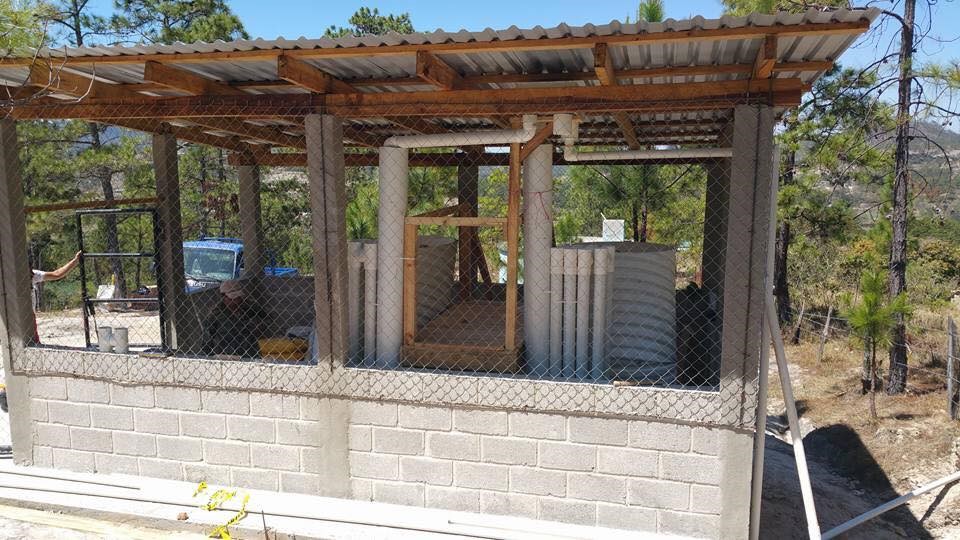
Fig. 85 Manzaragua water treatment plant using two of the AguaClara 1 L/s plants in parallel.
The plant performed very poorly from the first day of operation. The first attempted fix was to double the flocculator residence time by increasing the number of flocculator pipes (3 inch diameter by 1.5 m long) from 12 to 24. This improved performance, but the plant continued to perform poorly. A raw water sample was analyzed on May 30, 2018 and the following results were obtained.
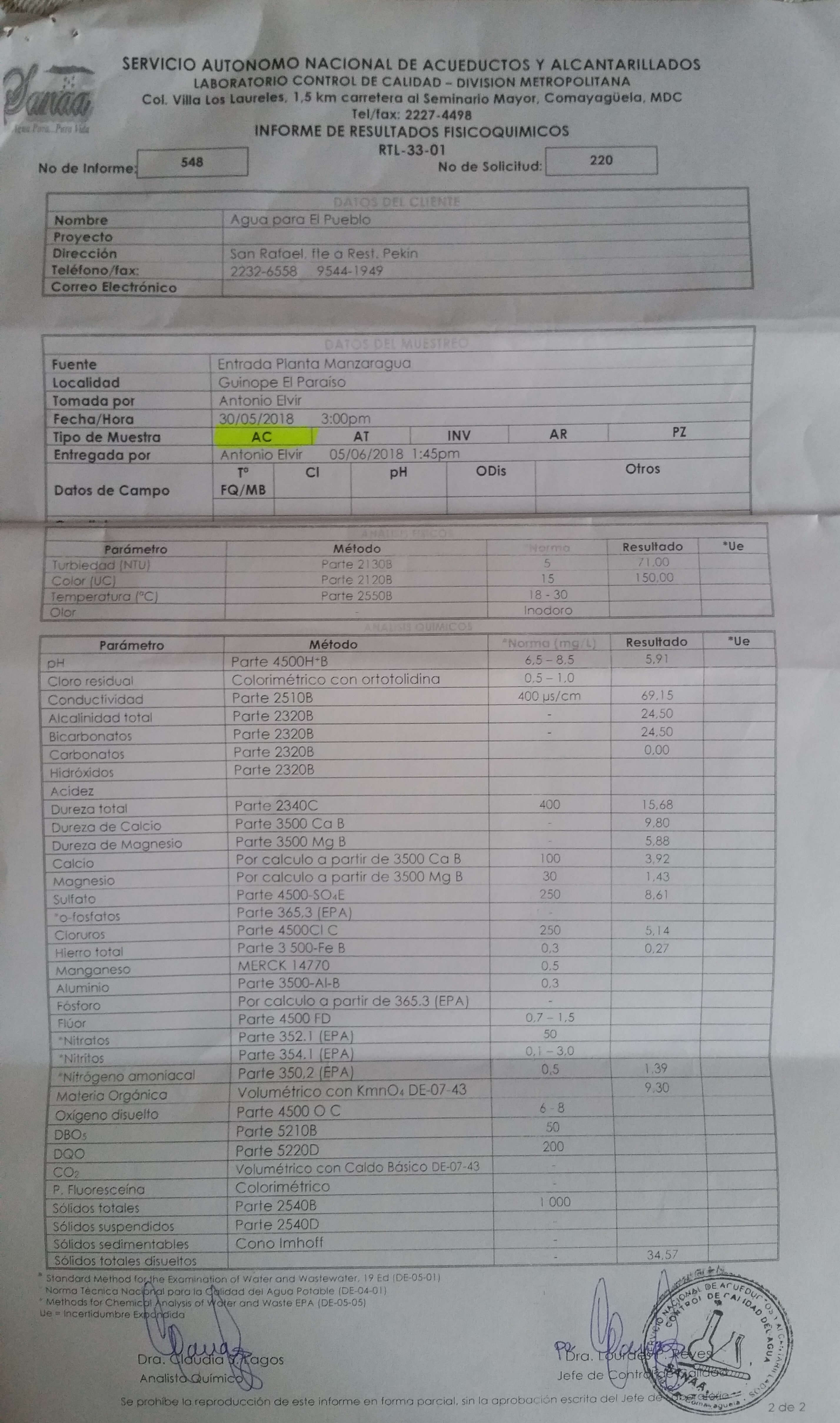
Fig. 86 Water quality analysis for Manzaragua.
Parameter |
Units |
Standard |
Results |
|---|---|---|---|
Turbidity |
NTU |
5 |
71 |
Color |
color units |
15 |
150 |
pH |
pH |
6.5 - 8.5 |
5.91 |
Conductivity |
\(\mu s/cm\) |
400 |
69.15 |
Alkalinity |
\(mg/L\) as \(CaCO_3\) |
24.5 |
|
Bicarbonates |
\(mg/L\) as \(CaCO_3\) |
24.5 |
|
Carbonates |
\(mg/L\) as \(CaCO_3\) |
0 |
|
Hardness |
\(mg/L\) as \(CaCO_3\) |
400 |
15.68 |
This water has high color which suggests a high concentration of dissolved organic matter. The pH is a clear problem because the pH is too low for the coagulant nanoparticles to precipitate. As the water sample has a pH of 5.91 a significant fraction of the coagulant will remain soluble.
Our goal is to determine how much base will need to be added to raise the pH. We do not have data on the optimal pH for treating high color water with PACl and so we will use pH 7 as the target.
At circumneutral pH (pH close to 7) the buffering capacity of the water is dominated by carbonate chemistry and specifically by the equilibrium between \({H_2}CO_3^{\star}\) and \(HCO_3^-\) . We will use the acid neutralizing capacity (reported as calcium carbonate alkalinity) and the pH from the sample analysis to estimate the total concentration of carbonates. We will not use the sample analysis carbonate concentrations because they can not be precisely correct.
We will find the amount of base that must be added using Equation (142).
Base/Acid |
\(Pi_{ANC}\) |
\(Pi_{CO_3^{-2}}\) |
|---|---|---|
\(Na_2CO_3\) or \(CaCO_3\) |
2 |
1 |
\(NaHCO_3\) |
1 |
1 |
\(NaOH\) |
1 |
0 |
\(HCl\) or \(HNO_3\) |
-1 |
0 |
\(H_2SO_4\) |
-2 |
0 |
For \(Na_2CO_3\) * \(\Pi_{ANC}\) = 2 we are adding \(CO_3^{-2}\) which is multiplied by two in the ANC equation because \(CO_3^{-2}\) can react with two protons. * \(\Pi_{CO_3^{-2}}\) = 1 because there is one mole of \(CO_3\) per mole of \(Na_2CO_3\)
Colab worksheet calculating the required base addition.
In following through the example it becomes apparent that the choice of base matters. The most efficient (on a mass or mole basis) base is \(NaOH\) because it doesn’t add any carbonates that don’t fully react with the hydrogen ions. The decision about which base to use will be influenced by economics, operator safety, and by whether additional carbonate buffering simplifies plant operation with changing raw water quality.
Chemical Name |
Common Name |
Chemical Formula |
|---|---|---|
Calcium carbonate |
Limestone or chalk |
\(CaCO_3\) |
Calcium hydroxide |
Slaked lime or hydrated lime |
\(Ca(OH)_2\) |
Calcium oxide |
Quicklime |
\(CaO\) |
The calcium bases are relatively inexpensive and have the disadvantage of lower solubility than sodium bases. Calcium carbonate has a low solubility, carbon dioxide is present in the atmosphere, and thus calcium carbonate precipitation limits the concentration that can be used for chemical feeds.

Fig. 87 Dose of three bases (in mole/L) required to achieve a target pH for the Manzaragua water. Carbonates provide more buffering and less change in the pH compared with \(NaOH\).
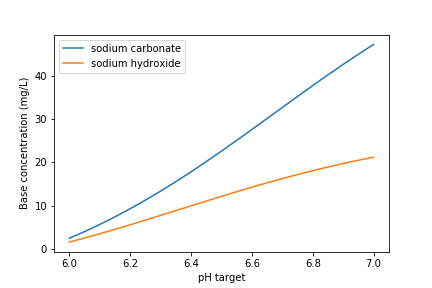
Fig. 88 Dose of two bases (in mg/L) required to achieve a target pH for the Manzaragua water. Carbonates provide more buffering and less change in the pH compared with \(NaOH\).
The required dose for each of the bases is summarized below.
Units |
\(NaOH\) |
\(NaHCO_3\) |
\(Na_2CO_3\) |
|---|---|---|---|
[mmoles/L] |
0.45 |
2.8 |
0.53 |
[mg/L] |
47.21 |
235.0 |
21.19 |
LFOM and Coagulant Injection Sizing
A water treatment plant that is treating 120 L/s of water injects the coagulant into the middle of the pipe that delivers the raw water to the plant and then splits the flow into 2 parallel treatment trains for subsequent flocculation. The pipe is PVC 24 inch nominal pipe diameter SDR 26. The water temperature is \(0^{\circ}C\). Estimate the minimum distance between the injection point and the flow split.
We will use a linear flow orifice meter with 20 cm of head loss. The first step is to determine the diameter of the LFOM.
Colab worksheet designing LFOM.
This analysis shows that the LFOM requires a 24 inch diameter pipe.
Example Problem: Energy Dissipation Rate in a Straight Pipe
Calculate the friction factor.
Use Equation (48) to estimate the mixing length in pipe diameters.
Convert to pipe length in meters.
Colab worksheet calculating the mixing length in pipe diameters
The previous analysis provides a minimum distance for sufficient mixing so that equal mass flux of coagulant will end up in both treatment trains. This assumes that the coagulant was injected in the pipe centerline. Injection at the wall of the pipe is a poor practice and would require many more pipe diameters because it takes significant time for the coagulant to be mixed out of the slower fluid at the wall. The time required for mixing at the scale of the flow in the plant is thus accomplished in a few seconds. This ends up being the fastest part of the transport of the coagulant nanoparticles on their way to attachment to the clay particles. Next we will determine a typical flow rate of coagulant. Aluminum concentrations for polyaluminum chloride (PACl) typically range from 1 to 10 mg/L. The maximum PACl stock solution concentration is about 70 g/L as Al.
Colab worksheet calculating the coagulant flow.
We can estimate the diameter of the injection port by setting the kinetic energy loss where the coagulant is injected into the main flow to be large enough to exceed the pressure fluctuations downstream of the LFOM. The amount of energy we invest in injecting the coagulant into the raw water is a compromise between having to raise the entire chemical feed system including the stock tanks to increase the potential energy and a goal of not having pressure fluctuations inside the LFOM pipe cause flow oscillations in the chemical dosing tube. Thus our goal is to have the kinetic energy at the injection point be large compared with the expected pressure fluctuations in the LFOM. Given that the head loss through the LFOM is often 20 cm, we expect the pressure fluctuations from turbulence to be a small fraction of that head loss. Thus we set the kinetic energy to be equivalent to 2 cm.