AguaClara Hydraulic Flocculation Model

The AguaClara hydraulic flocculation model was developed over 15 years of extensive laboratory and field research and is based on the physics of interactions between particles in the raw water, dissolved organic molecules, and coagulant nanoparticles in a shear flow. The AguaClara model is based on the physics of these interactions and is the first non-empirical flocculation model.

2005 - We used conventional guidelines based on velocity gradient to design the first low flow vertical flocculator

2010 - We designed using energy dissipation rate and accounted for the nonuniformity of the energy dissipation rate (\(\theta\) = 15 minutes)

2015 – We added obstacles to decrease the distance between expansions to make all of our flocculators have maximum collision efficiency (\(\theta\) = 8 minutes)

2016 – Learned that particle/floc collisions are dominated by viscous shear (not by turbulent eddies). Began designing flocculators based on a target head loss of 40 cm. Used a \(G\theta\) of 37,000.

2017 - Designed a pipe flocculator for the 1 L/s plant with a \(G\theta\) of 20,000 and a residence time of about 100 s.

2020 - Realized that flocs with a high fraction of organic matter have a lower density and thus must be larger to settle in the clarifier. This requires a lower velocity gradient in the flocculator and the inlet to the clarifier.

Conventional vs AguaClara Flocculation

Table 15 Conventional vs AguaClara flocculation

Characteristic	Conventional - Mechanical	AguaClara - Hydraulic
Goal	produce large flocs to be captured by sedimentation	reduce the concentration of primary particles
Residence time (min)	30	2 to 7.5
Velocity gradient (Hz)	20 - 180	100+
\(G\theta\)	50,000 - 250,000	20,000 - 37,000
Velocity gradient variability	8 (highly variable)	approximately 1.4
reactor type	approaching completely mixed	approaching plug flow

#references Coagulation and Flocculation in Water and Wastewater Treatment, iwapublishing

Collisions in Shear Flow

Given that hydraulic flocculators approach plug flow conditions it is reasonable to assume that at any given location in the flocculator there is a predominance of one size of flocs. Thus collisions between similar sized flocs are most likely because that is what is present. There is also a hydrodynamic reason why collisions between similar sized flocs are favored.

In a shear flow the particles rotate and a boundary layer is created all around the rotating particles. The boundary layer prevents collisions between different sized particles (see Fig. 115) because the smaller of the two particles is unable to extend through the boundary layer of the larger particle. Only particles that are large enough to extend through each other’s boundary layers can collide (see Fig. 116). Thus the particles must be similar in size because the boundary layer also scales with the diameter of the particle.

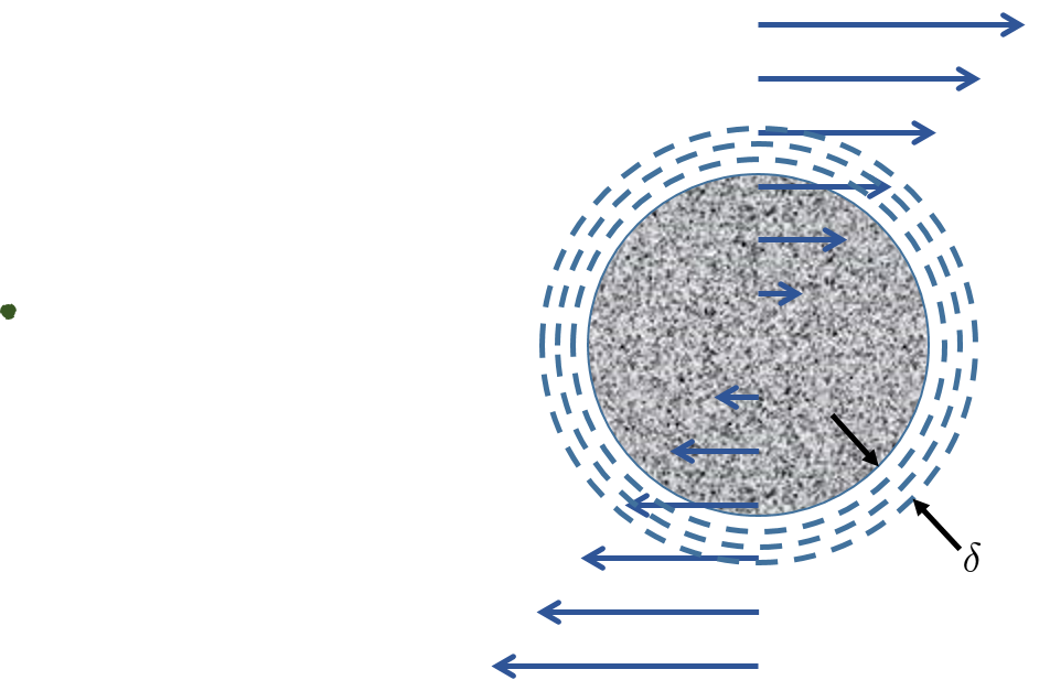
Fig. 115 Particles that are very different in size don’t even get close enough to make contact because of the boundary layer around the larger particle. This is because the thickness of the boundary layer also scales with the diameter of the particle.

Collisions between similar sized particles are possible because the particles are able to extend through the boundary layers.

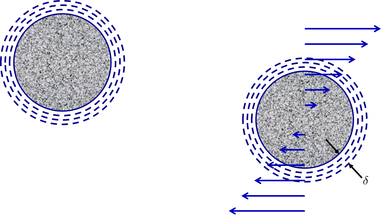
Fig. 116 In a shear flow the particles rotate and a boundary layer is created all around the rotating particle. Similar sized particles are able to extend through the boundary layers and make contact.

The rotating boundary layers in a shear flow limit collisions to similar sized particles. Given that flocculation is an environment specifically designed to create fluid shear it is reasonable to assume that only collisions between similar sized particles are able to occur. This simplifies the Smoluchowski equation tremendously.

Floc Formation

For simplicity of modeling let’s assume that flocs repeatedly double in size as suggested by the movie in Fig. 96. In that case, the number of primary particles in a floc is given by

(167)\[ n_{primary} = 2^{n_{collisions}}\]

If we assume (and we will show this assumption to be wrong in the next step) that the floc volume is directly proportional to the total volume of the primary particles in the floc, then we can rearrange (167) to solve for the number of sequential collisions required to increase the number of primary particles by a factor of 1000,000,000.

(168)\[ n_{collisions} = \frac{log(n_{primary})}{log(2)}\]

See here for the code to determine the number of collisions

30 sequential collisions would be required to produce a floc that contains 1 billion primary particles.

As flocs combine they don’t coalesce like mist turning into rain drops. Instead they form loose aggregates that contain a higher and higher fraction of water in the voids between the solid primary particles.

Although the obvious flocculation advantage is that it produces larger aggregates that are easier to remove, it is also possible (this is a hypothesis that needs testing) that a difference in a physical property between primary particles and flocs plays a role in enhanced removal of flocs in floc filters and filters. For example, the many relatively weak connection points between the primary particles in the flocs enables the flocs to deform. It is possible that deformation plays an important role right at the moment of collision. Presumably the bond strength required to lock the colliding particles together is less if the particles can deform as they are colliding.

The size change produced by flocculation is dramatic. Clay particles and pathogens have sizes that are order \(\mu m\) and they combine to form flocs that are order \(mm\). A thousand fold increase in diameter suggests a billion fold increase in volume.

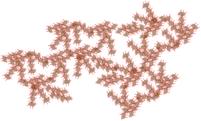
Fig. 117 The amount of water contained within a volume defined by the floc increases as the flocs grows.

One of the mysteries of flocculation has been why it is such a slow process, requiring 30 minutes according to conventional design, and yet it appears to be a very rapid process. Plant operators observe that with high raw water turbidities that they can see flocculation progressing after about 0.5 minutes of flocculation. We can estimate the collision potential, \(G\theta\) that corresponds to making visible flocs.

\[\bar G = \sqrt{ \frac{g h_e}{\theta \nu}}\]

Colab worksheet to create visible flocs during high turbidity

Here initial flocculation is visible at a \(G\theta\) of less than 3000. Given that flocculation is visible at this low collision potential, it is unclear why recommended \(G\theta\) are as high as 100,000. This is one of the great mysteries that motivated the search for a flocculation model that is based on physics and consistent with laboratory and field observations.

Collision Time

Now that we know that the collisions are controlled by viscosity we can begin formulating a model that describes the long distance random walk. The long range transport is assumed to be the rate limiting step. We model a system of two particles where one particle is held fixed and we observe the second particle’s random motion. It may be helpful to visualize this by playing the video inside your mind in reverse starting from the moment of the collision. That way you know which two particles to follow! The random walk is illustrated in the video in Fig. 118.

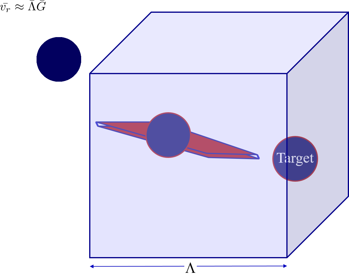
Fig. 118 The red volume represents the potential end zone of the random walk that will slide into a collision with a short straight slow walk. The wandering particle sweeps through a volume of water equal to the volume occupied by a single particle.

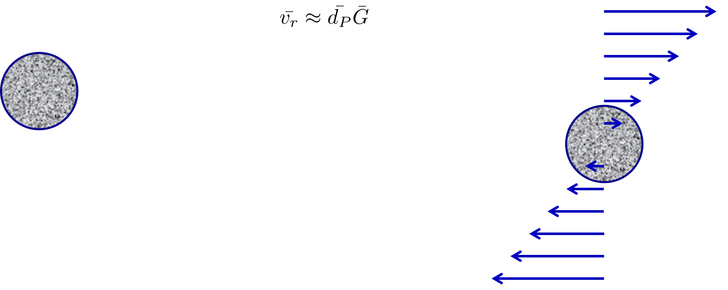
Fig. 119 The final approach is the slow, straight path to the collision.

The volume cleared by the wandering particle is proportional to the area defined by a circle with diameter = sum of the particle diameters. This is because the wandering particle with strike the stationary particle if the wandering particle’s center is anywhere within a diameter of the center of the stationary particle.

\[{\forall_{\rm{Cleared}}} \propto \pi \bar D_P^2\]

The volume cleared is proportional to time

\[{\forall_{\rm{Cleared}}} \propto t\]

The volume cleared is proportional to the relative velocity between the two particles.

\[{\forall_{\rm{Cleared}}} \propto \bar v_r\]

We use dimensional analysis to get a relative velocity for the long range transport controlled by shear. The relative velocity between the two particles that will eventually collide is assumed to be proportional to the average distance between the two particles.

The assumption that the relative velocity scales with the average distance between clay particles leads to the following steps. The first step is just a proposed functional relationship. We could also have jumped to the assumption that the relative velocity is a function of the length scale and the velocity gradient.

\[\bar v_r = f \left( \bar \varepsilon ,\nu ,\bar \Lambda \right)\]

In a uniform shear environment the velocity gradient is linear. Thus the relative velocity must be proportional to the length scale.

\[\bar v_r = \bar \Lambda f \left( \bar \varepsilon ,\nu \right)\]

The only way for \(\bar \varepsilon\) and \(\nu\) to produce dimensions of time is to combine to create \(1/\tilde{G}\).

\[\bar v_r \approx \bar \Lambda \tilde{G}\]

The volume cleared, \({\forall_{\rm{Cleared}}}\) must equal the volume occupied by one particle, \({\forall_{\rm{Surround}}}\) for a collision to occur. Combining the three equations for \({\forall_{\rm{Cleared}}}\) and the equation for \(v_r\) we obtain the volume cleared as a function of time.

\[\bar \Lambda^3 = {\forall_{\rm{Surround}}} = {\forall_{\rm{Cleared}}} \approx \pi \bar D_P^2 \bar \Lambda \tilde{G} \bar t_c\]

Where:

\(\bar t_c\) is the average time required for a collision between two particles

Solving for the collision time we obtain

(169)\[\bar t_c \approx \frac{\bar \Lambda^2}{\pi \bar D_P^2 \tilde{G}}\]

In summary, a relationship for the mean time between collisions \(\bar{t_{c}}\) was found by proposing an average condition for a collision, successful or unsuccessful, to occur. To define this condition, it was assumed that each primary particle on average occupies a fraction of the reactor volume, \(\bar{V}_{Surround}\), inversely proportional to the number concentration of particles. Furthermore, prior to a collision, a particle on average sweeps a volume, \(\bar{V}_{Cleared}\), proportional to \(\bar{t_c}\) and to the mean relative velocity between approaching particles, \(\bar{v}_r\). As an average condition, it was posited that for each collision, \(\bar{V}_{Cleared}\) must equal \(\bar{V}_{Surround}\). From this, a relationship for a characteristic collision time, \(\bar{t_c}\), was obtained:

The change in the number of particles with respect to time is proportional to attachment efficiency and the time required per collision.

(170)\[ \frac{dN_c}{dt}== \frac{\alpha}{t_c}\]

The collision rate [PCWSL16] can be obtained by substituting Equation (169) into Equation (170).

(171)\[ \frac{dN_c}{dt}=\pi\bar{\alpha}\frac{\bar{D}_{P}^2}{\bar \Lambda^2} \tilde{G}\]

where \(\tilde{G}\) is the Camp Stein velocity gradient.

Because the flocculation performance equation will ultimately track particle concentration, the concentration of primary particles, \(C_{P}\), was substituted for \(\bar \Lambda\) using

(172)\[ \bar \Lambda^3=\frac{\pi}{6}\frac{\rho_{P}}{C_{P}}\bar{D}_P^3,\]

where \(\rho_{P}\) is the characteristic density of primary particles. Equation (172) can be substituted into Equation (171) to result in:

(173)\[ dN_{c}=\pi\bar{\alpha}\left(\frac{6}{\pi}\frac{C_{P}}{\rho_P}\right)^{2/3}\tilde{G}dt.\]

Equation (173) reveals that \(\frac{dN_c}{dt}\) increases with \(C_P\) and \(\bar{\Gamma}\). During flocculation \(C_P\) will decrease and thus \(\frac{dN_c}{dt}\) will also decrease.

Coagulant Nanoparticles and Primary Particles

Continuing from [PCWSL16], the above Lagrangian differential relationships are further developed to become integrated performance prediction equations. Equation (173) cannot be integrated as written because the concentration of primary particles is expected to change with each collision, and thus that relationship must be specified. During the average time required for one collision it is expected that approximately \(e^{-1}\) of the particles will undergo at least one collision. The time required for a collision will change as flocculation proceeds as the average distance between primary particles increases. The rate of loss of primary particles due to successful collisions will be first order with respect to the number of successful collisions.

(174)\[ \frac{dC_{P}}{dN_{c}}=-kC_{P},\]

where \(k\) is an experimentally-derived constant that physically represents the portion of the primary particles that become settleable particles on average after each collision time, \(\bar{t_c}\), and will depend, in part, upon the design capture velocity, \(\bar v_c\), used for sedimentation. Since \(\bar{t_c}\) increases over time as \(\bar \Lambda\) increases, the above formulation is not proportional to \(\frac{dC_P}{dt}\). Physically, Equation (174) states that, with each progressive primary particle collision, \(C_P\) decreases by some proportion. Further, Equation (174) states that this decrease is directly proportional to \(C_P\). With each successive successful collision, the absolute reduction in \(C_P\) is less than the prior one. The value of \(k\) is expected to be less than 1, because not all primary particles will have a collision and grow to a size with a terminal velocity greater than \(\bar v_c\) in the average time required for a collision.

Having Equation (174), the next step is to substitute it into Equation (173) and integrate. Solving Equation (174) for \(dN_{c}\), substituting it into Equation (173) and rewriting the equations in terms of primary particles results in Equation (175),

(175)\[ \frac{dC_{P}}{-kC_{P}}=\pi\bar{\alpha}\left(\frac{6}{\pi}\frac{C_{P}}{\rho_P}\right)^{2/3}\tilde{G}dt,\]

It is interesting to note that rearranging Equation (175) in terms of \(\frac{dC_P}{dt}\) gives a \(C_P\) exponent of \(\frac{5}{3}\). Previous flocculation rate equations were second-order, but the observed flocculation rate was less than second-order [BL13]. The slight deviation from an exponent of two comes from the assumption of [PCWSL16] that relative velocity between colliding particles scales with \(\Lambda\) rather than \(d_P\). This is to say that, in dilute suspensions characteristic of raw water, where particles are separated by \(\bar \Lambda\gg \bar{D}_P\), the majority of \(\bar{t_c}\) is spent with the distance between particles characterized by \(\bar \Lambda\) instead of \(\bar{D}_P\). The time required for the final approach for a collision is hypothesized to be insignificant compared the time for \(\bar{V}_{Cleared}\) to equal \(\bar{V}_{Surround}\).

From Equation (175) it is possible to integrate and obtain equations for flocculation performance. After separation of variables, one side of the equation is integrated with respect to time from the initial time (\(t=0\)) to the time of interest, generally taken to be the mean hydraulic residence time (\(t=\theta\)). The other side of the equation is integrated with respect to the concentration of primary particles from the value at the initial time (\(C_{P_0}\)), equivalent to the initial concentration of primary particles, to the concentration of primary particles at the time of interest (\(C_{P}\)). The integral becomes:

(176)\[ \frac{1}{\pi}\left(\rho_{P}\frac{\pi}{6}\right)^{2/3}\int_{C_{P_0}}^{C_{P}}C_{P}^{-5/3}dC_{P}=-k\bar{\alpha}\tilde{G}\int_0^\theta dt.\]

The integral on the left hand side assumes that \(\rho_{P}\) does not change as \(C_P\) changes. One assumption on the right side is that \(\bar{\Gamma}\), of which \(\bar{\alpha}\) is a function, does not vary with \(t\). This requires that adsorption of coagulant to colloidal particles in rapid mix be fast enough to be approximated as completed by the beginning of flocculation. This assumption may not be valid for high rate flocculators especially under conditions of low \(C_{P_0}\). Further work on the rate and efficacy of coagulant nanoparticle attachment to primary particle surfaces is needed.

The other assumption on the right hand side is that the mean velocity gradient, \(\tilde{G}\), does not change over the course of the flocculation process. In mechanically-mixed flocculators, the use of a simple spatial average is not reasonable, as the velocity gradient changes dramatically from the bulk flow to the tip of the impeller blade and individual particles follow different paths that expose them to different velocity gradient zones in different sequences and durations [BB98]. The distribution of residence times in a mechanical flocculator would also need to be taken into account for the integration. For baffled hydraulic flocculators, on the other hand, the use of the spatial average, \(\tilde{G}\), and considering it constant with \(t\) is generally a reasonable approximation, as mixing energy in a well-designed hydraulic flocculator is rather uniformly distributed spatially, the zones of higher energy dissipation rate after the baffles do not vary appreciably with time when operating at a constant flow rate, and all particles have similar residence times in the flocculator.

Integration of Equation (176) gives:

(177)\[ \frac{3}{2\pi}\left(\rho_{P}\frac{\pi}{6}\right)^{2/3}\left(C_{P}^{-2/3}-C_{P_0}^{-2/3}\right)=k\bar{\alpha}\tilde{G}\theta.\]

This can be put in terms of \(\bar \Lambda\) for simplicity by using Equation (172) and rearranging in terms of the familiar Camp-Stein parameter, \(\tilde{G}\theta\), to be

(178)\[ \tilde{G}\theta = \frac{3}{2}\frac{{\left( {{\bar \Lambda ^2} - \bar \Lambda_0^2} \right)}}{{k\pi\bar{\alpha} \bar{D}_P^2}}.\]

Equation (178) gives guidance for flocculator design in that higher values of \(\tilde{G}\theta\) are needed for flocculators to achieve greater changes in \(\bar \Lambda\) (or \(C_P\)) or to overcome low \(\bar{\Gamma}\). It should be noted that the \(\bar \Lambda_0\) term in Equation (178) will generally be very small compared to the \(\bar \Lambda\) term for most flocculation scenarios. In this case the initial particle separation distance, \(\bar \Lambda_0\) can be considered negligible. While simplifying the equation, this also gives the result that flocculators must be designed not so much for the particle concentrations they will receive but for the particle concentrations they are intended to produce.

Modifying Equation (178) to be in terms of \(C_P\) produces:

(179)\[ \tilde{G}\theta = \frac{3}{2k\pi\bar{\alpha}}\left(\frac{\pi}{6}\frac{\rho_P}{C_P}\right)^{2/3}.\]

Solving Equation (179) for \(C_P\) we obtain

(180)\[ C_{P} = \frac{ \left( {\frac{\pi}{6}{\rho_{P}}} \right)}{\left( \frac{2}{3} \pi k \tilde{G}\theta \alpha \right)^\frac{3}{2}}.\]

Experimental Protocols

Equation (177) was tested under turbulent conditions. The design scheme chosen to meet these requirements was a tube flocculator, illustrated in Fig. 120 and described in [PCWSL16]. This tube flocculator operated in the turbulent flow regime, which for pipe flow means that \(Re>4,000\) [Gra95]. The change in mean energy dissipation rate due to any modification to the system was approximated by

(181)\[ \bar{\varepsilon}=\frac{gh_\ell}{\theta},\]

where \(g\) is the acceleration due to gravitational force and \(h_\ell\) is the head loss across the flocculator. As mentioned previously, the use of \(\bar \varepsilon\) assumes that the energy dissipation rate throughout the flocculator is completely uniform so that it can be represented with a simple spatial average rather than a weighted average accounting for the proportion of the flow passing through different zones of energy dissipation rate. This approximation requires that the majority of energy dissipation (represented by head loss) is due to fluid shear (minor loss) in the bulk flow. If the head loss across a flocculator were primarily as a result of shear on the reactor walls (major loss), only a small fraction of the flow would experience this energy dissipation rate in the near-wall zone, and estimating the mean energy dissipation rate by this method would be invalid.

It is hypothesized, however, that the constrictions in the tube flocculator created submerged free jets downstream, generating fluid shear across the cross section of the flow [PCWSL16]. This hypothesis is supported by a calculation of the head loss due to wall shear using the Darcy-Weisbach Equation [Gra95]. The turbulent tube flocculator would be expected to have a total head loss of around 7 cm if only wall shear were present, but an average head loss of 90 cm was measured across the flocculator by means of a differential pressure sensor, indicating that significant fluid shear is present.

Referring to Equation (181), changing the head loss by changing the constriction of the tubes or changing the water elevation difference across the flocculator would change the energy dissipation rate. Likewise, either of the above two modifications would change the mean hydraulic residence time in the flocculator. This could also be accomplished by changing the length of the flocculator.

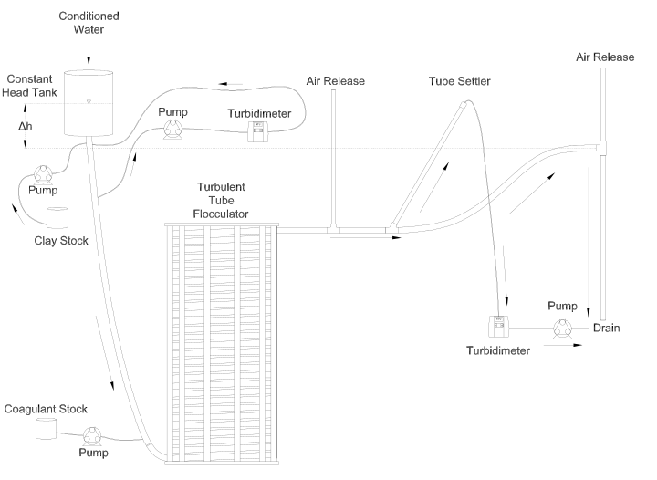
Fig. 120 Diagram of Turbulent Tube Flocculator adapted from [PCWSL16] with modifications made to the outlet weir system and the addition of strong base solution.

Fig. 120 illustrates the process sequence used in this study. At the beginning of the process, tap water from the Cornell University Water Filtration Plant came into the system with, on average, a pH of 7.67, a turbidity of 0.056 nephelometric turbidity units (NTU), a total hardness of 150 mg/L, a total alkalinity of 140 mg/L, and a dissolved organic carbon (DOC) concentration of 1.80 mg/L [BPMWSCIWSCUWS16]. This water was temperature-controlled by means of a PID (proportional-integral-derivative) controller, which regulated the relative fractions of hot water and cold water used to maintain the level in the constant head tank. The temperature-controlled water was passed through a granular activated carbon (GAC) filter to reduce the effect of dissolved organic matter (DOM) on experimental results. The water was then sent to the constant head tank, where it was bubbled with air to strip out supersaturated dissolved gases that might come out of solution during the experiment, resulting in formation of bubbles.

From the constant head tank, this conditioned water was delivered to the turbulent tube flocculator. Before entry to the flocculator, the water was set at a constant primary particle concentration by means of a computer-controlled peristaltic pump that introduced a concentrated kaolinite clay suspension (R.T. Vanderbilt Co., Inc., Norwalk, Connecticut) of about 250 g/L. A fraction of the mixed flow was sampled by a peristaltic pump and analyzed for turbidity with an HF Scientific MicroTOL turbidimeter at a distance of greater than ten diameters downstream from the clay input and then reintroduced at the point where clay suspension was added. This turbidity reading was input into a PID control system which determined the speed of the clay pump according to the discrepancy between the influent turbidity and the experimental target value.

Along with the clay, strong base (NaOH) manufactured by Sigma-Aldrich (St. Louis, MO) was added upstream of the flocculator with a peristaltic pump to keep the pH of the water at \(7.5\pm0.5\), which was the criterion set for the pH in these experiments. In the winter, the pH of the tap water dropped close to 7, and so sufficient NaOH was added to account for seasonal variations in the natural base-neutralizing capacity (BNC) of the water and to raise the pH above 7 to around 7.5. This base addition was also sufficient to neutralize the acidity of the polyaluminum chloride (PACl) coagulant used for this study, which had been found to impact the solubility of PACl at high doses. Base doses were calculated to account for the normality of the PACl solution, based on a titration which found that the PACl solution was approximately 0.025 equivalents of strong acid per gram as Al.

Just prior to entering the flocculator, PACl coagulant (PCH-180) manufactured by the Holland Company, Inc. (Adams, Massachusetts) was added to the flow by a computer-controlled peristaltic pump which varied the coagulant dose between experiments. After entering the system, the coagulant then entered a small orifice used to accomplish rapid mix by forming a jet downstream. From there, the suspension traveled up through the flocculator made of 3.18 cm (1.25 in) inner diameter tubing. Within the flocculator, the fluid passed through constrictions in the tubing that caused the flow to contract, resulting in flow expansions afterward and achieving increased mixing and energy dissipation.

After leaving the flocculator, the flow passed a vertical tube with a free surface that served as an air release. This removed bubbles in the system so that they would not interfere with settling or analysis of the flocs. A portion of the flow was then diverted for sedimentation by means of a peristaltic pump up a clear one-inch PVC pipe angled at \(60^{\circ}\). The flow rate through the pump was selected based on the dimensions of the tube and its angle to achieve a desired capture velocity, \(\bar v_c\). The supernatant from this tube settler was passed through an HF Scientific MicroTOL nephelometric turbidimeter to record the effluent turbidity for the duration of the experiment. Recording the settled effluent turbidity made it possible to calculate the \(pC^*\) term in Equations (177) (in terms of primary particles) and also made possible comparison with data from [SWSL14].

After data from the settled flocs had been collected, the flow from the effluent turbidimeter was sent to the drain along with the bulk flow. The bulk flow traveled past a second air release before exiting the drain. The air release gave the flow exiting the drain a free surface as it flowed over the exit weir so that the exiting water developed into a supercritical flow. Thus, the flow over the weir was not influenced by the flow downstream of the free surface, and the flow rate could be controlled by adjusting the elevation of the free surface before the drain. The outlet weir was a 1-1/4” PVC pipe within an upright 3” clear pipe, which were joined by a flexible coupling adapter. The effluent water accumulated in the clear outer pipe until it reached the elevation of the top of the inner pipe and flowed down through it. The flow rate could be adjusted by loosening the flexible coupling so that the elevation of the top of the inner pipe could be adjusted. As the bulk flow exited down out of the inner pipe to the drain, it passed over a glass electrode sensor to measure pH.

Results

The above process was used to conduct the experiments to test the applicability of Equation (177) in turbulent flocculation. The influent turbidity was set at a constant of 900 NTU. The mean energy dissipation rate was about 21.5 mW/kg, which resulted from choosing a flow rate of about 110 mL/s so that the Reynolds number was just above 4,000. These values were chosen to ensure viscous-dominated turbulent initial conditions. For these experiments, coagulant doses ranged from 0.05 to 98 mg/L as Al. A \(\bar v_c\) of 0.12 mm/s was used for all experiments. Data from these nominally viscous experiments are shown in Fig. 121 as a function of coagulant dose.

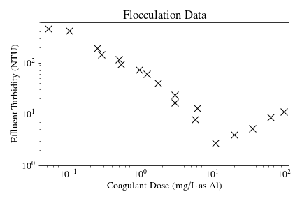
Fig. 121 Effluent turbidity as a function of coagulant dose for experiments performed with influent turbidity of 900 NTU, velocity gradient of 147 Hz, and hydraulic residence time of about 413 s.

The data shown in Fig. 121 were compared with the viscous model, as shown in Fig. 122. In this graph, the data are plotted in terms of Equation (177) and its corresponding composite parameter taken from Equation (171),

(182)\[ N_{c}\propto\bar{\alpha}\theta \tilde{G}\phi_0^{2/3}.\]

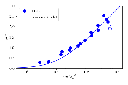
Fig. 122 Fit of Equation (177) to data from \(Re\approx 4,000\) experiments. Hollow points indicate data not used in fitting the model.

At the highest values, however, a marked decrease begins. For these graphs, the model fits were done for all points where increasing performance was seen, because the model does not currently include a mechanism for the decreasing performance. The values for \(k\) were determined by the Levenberg-Marquardt algorithm, and the value for the model was 0.030. The \(R^2\) value for the fit is 0.958 and the sum of squared errors is 0.228 (mean pC* error of 0.128).

From the values given previously, the ratio \(\frac{\bar \Lambda_0}{\bar{\eta}}\) can be calculated for the experimental conditions. Equation (172) can be used to compute (\(\bar \Lambda_0\)). For these experiments, \(\bar{D}_P\) is taken to be the average diameter of kaolinite clay particles, found by [WZL+15] and [SWSL15] to be 7 \(\mu m\). The concentration can be converted from NTU to the necessary mass/volume (mg/L) unit by using as a proportion the measurement reported by [WZL+15] of 68 NTU for 100 mg/L of kaolinite clay. Last, the density was assumed to be 2.65 g/\(cm^3\) for kaolinite.

For flocculation in laminar flows, data were used from the work of [SWSL14]. Fig. 123 shows Equation (177) fit to results for a capture velocity of 0.12 mm/s at two hydraulic residence times, five influent turbidity values and a range of coagulant doses. [SWSL14] showed that the projected x-axis intercept of the linear region of the data (with a log-log slope of 1 according to her plotting of the data) was proportional to the capture velocity used for sedimentation. Correspondingly, \(k\) is expected to be a function of capture velocity.

Fig. 123 Fit of Equation (177) to laminar flocculation data from [SWSL14].

Referring to Fig. 123, Equation (177) fits the data from [SWSL14] well with a \(k\) value of 0.027. The resulting \(R^2\) for this fit is 0.844. The sum-squared error is 5.03, giving an average pC* error of 0.034 for the fit.

Discussion

The goodness of fit seen in Fig. 122 and Fig. 123 indicate that the model captures the important mechanisms governing flocculation performance for a wide range of coagulant doses in both laminar and turbulent hydraulic flocculation. One of the challenges in fitting the data pertained to the assumption made for the characteristic diameter of PACl precipitate clusters, \(\bar{D}_C\). This value has significant influence on the value of \(\bar{\Gamma}\), which in turn influences the values of the composite parameter (Equation (182)).

It is known that PACl contains aluminum monomers and oligomers as well as \(\mathrm{Al_{13}}\) and \(\mathrm{Al_{30}}\) nanoclusters, with the larger \(\mathrm{Al_{30}}\) nanoclusters having a diameter of 1 nm and a length of 2 nm [MCM+12]. It has been found, however, that the components of PACl self-aggregate and go on to form larger clusters [SWSL13]. For these experiments, the value of \(\bar{D}_\mathrm{C}\) was chosen based on sizing experiments performed by Garland (2017) with a Malvern Zetasizer Nano-ZS to analyze a 138.5 mg/L (as Aluminum) solution of PACl.

A limitation of the model can be seen in the data in Fig. 122 at higher values of the composite parameters. After increasing steadily for all of the preceding range of coagulant doses, the performance began to decline after the dose of 10.9 mg/L as Aluminum. A simple hypothesis for the decline in performance (which corresponds with an effluent turbidity increase over the five data points from 2.7 NTU to 11.1 NTU) is that an increase in free PACl nanoparticles made a significant contribution to the effluent turbidity. As the PACl concentration increased, the coverage of reactor and clay platelet surfaces by coagulant became more complete and the free coagulant concentration also increased. With very high coagulant doses like the ones used in the upper end of the experimental range, it is possible that the formation of PACl self-aggregates was favorable, increasing the turbidity of the suspension. Indeed, calculation of the volume fraction for the 10.9 mg/L experimental PACl dose gives a volume fraction value (for clay and coagulant combined) of \(6.1\times10^{-4}\), while for the highest dose of 98 mg/L as Al, the value was \(8.3\times10^{-4}\), a 37% increase due solely to the increased contribution of PACl precipitates.

Another possibility is that as \(\bar{\Gamma}\) increases above 0.5, the resulting flocs are increasingly formed by PACl-PACl bonds instead of by PACl-kaolinite bonds. If the PACl-PACl bonds are weaker than PACl-kaolinite bonds, it is possible that attachment efficiency decreases for high \(\bar{\Gamma}\). The weakness of PACl-PACl bonds compared with PACl-kaolinite bonds is suggested by the relative charges of PACl and kaolinite. While PACl precipitate surfaces are positively charged, the surfaces of kaolinite are mostly negatively charged [WZL+15]. Therefore, it follows that PACl precipitates will likely have more affinity for kaolinite surfaces than for other PACl precipitates. The \(\bar{\Gamma}\) calculated for the peak performance was 0.52, and so it is possible that performance decreased past this point because the strength of bonds for experiments at higher doses were weaker.

Applying the AguaClara flocculation model to the design of a hydraulic flocculator indeed gives reasonable results. Assuming that a flocculator is expected to receive sufficiently high turbidities that the influent concentration can be neglected, Equation (179) can be used. In order for it to treat to a settled effluent of 3 NTU (pre-filtration) with sufficient PACl to achieve a surface area coverage fraction of 0.5, it would need to have a \(\tilde{G}\theta\) of 99,600. [DC08] give the range of \(\tilde{G}\theta\) values pertinent to flocculation of high turbidities as between 36,000 and 96,000, so this result is reasonable. This analysis does not account for removal of particles in a floc filter that would enable use of a lower value of \(\tilde{G}\theta\).

Regarding flocculator design, recommended values of \(\tilde{G}\) in flocculation range from \(10\:\mathrm{\frac{1}{s}}\) to \(100\:\mathrm{\frac{1}{s}}\), which correspond to \(\bar{\varepsilon}\) values of about 0.1 to 10 mW/kg [ML00]. However, there is evidence that higher velocity gradients are advantageous, as found by [GWSL16] as well as the work done in this study, which made use of energy dissipation rates of about 22 mW/kg. For hydraulic flocculators, at least, designers should consider using higher energy dissipation rates than conventionally used, since they have a much lower ratio of maximum to average energy dissipation rate, leading to less floc breakup at high energy dissipation rates compared to mechanically mixed flocculators.

The assumption that nonsettleable particle removal is proportional to primary particle removal appears to be supported by the goodness of fit supplied by the AguaClara flocculation model to the data (see Fig. 122). This assumption is likely included in the values of \(k\) fit by the model. A mechanistic understanding of \(k\) will require that the proportionality between nonsettleable and primary particles be understood explicitly. It is possible that \(k\) is a function of rapid mix effectiveness, and since \(k\) predicts \(pC^*\), it will also be dependent on \(\bar v_c\). Future experiments at varying \(\bar v_c\) are planned. Currently, \(\bar{\alpha}\) is calculated assuming that coagulant nanoparticle attachment to the primary particles was accomplished very early on in the flocculator, but if colloid coating by coagulant nanoparticles is dependent upon diffusion rather than exclusively on hydraulic shear, it will be a function of time in addition to \(\tilde{G}\theta\), making flocculation less effective at high flow rates. Additionally, the use of \(\bar{\varepsilon}\) (or \(\tilde{G}\)) assumes a uniform energy dissipation rate in the flocculator. Any spatial deviation in the laboratory flocculator from a uniform energy dissipation rate would have had an impact on the values of \(k\) relative to their theoretical values, which are dictated by the rate of conversion of primary particles to flocs.

Summaries

We developed a model that predicts hydraulic flocculator performance. Regardless of whether the flow is laminar or turbulent, viscous forces control the relative velocities between particles on a collision path, and the performance equation is \(pC^*=\frac{3}{2}\log_{10}\left[\frac{2}{3}\left(\frac{6}{\pi}\right)^{2/3}\pi k\bar{\alpha}\tilde{G}\theta\phi_0^{2/3}+1\right]\).

Model predictions were compared with data from [SWSL14]. To validate the first equation and the second equation in turbulent flow, experiments were conducted in turbulent flow for initial conditions of \(\frac{\bar \Lambda}{\bar{\eta}}<1\). It was found that the viscous equation was slightly more suitable in these conditions. Until further work is done on delineating the relative predominance of viscous and inertial forces over the range of turbulent flocculation conditions, the authors recommend using the AguaClara flocculation model. For design purposes, this model indicates that flocculator design is more sensitive to the desired effluent concentration of particles than the range of influent concentrations that might be encountered. This study also supports the use of higher energy dissipation rates (or velocity gradients) than conventionally recommended for hydraulic flocculators. Further work is needed to characterize the functional dependence of \(k\) on capture velocity and energy dissipation rate, as well as the relationship between the final concentrations of primary and primary particles.

Geometric Explanation of the Effects of Humic Acid on Flocculation

Dissolved organic matter (DOM) is ubiquitous in natural waters and has considerable influence on drinking water treatment, since the presence of DOM can create a need for increased coagulant doses in addition to being a precursor of disinfection byproducts (DBPs). This work evaluated use of polyaluminum chloride (PACl) as a coagulant for a synthetic water to determine the effect of DOM on the settled effluent turbidity. The research employed the hydraulic flocculation performance model previously discussed and made additions to the model algorithm to incorporate the effects of humic acid on flocculation of inorganic particulate matter. Data were obtained using a laminar-flow tube flocculator and a lamellar tube settler. Two adjustable model parameters were used to fit data, one related to the capture velocity used for sedimentation, and one that estimated the average size of dissolved humic acid molecules. The modified model that accounted for the presence of humic acid was able to independently predict the experimental results from 60 experiments at a different influent turbidity. This section is based on Observations and a Geometric Explanation of the Effects of Humic Acid on Flocculation published in Environmental Engineering Science in 2019 (DOI#10.1089/ees.2018.0405), and the reader is encouraged to consult this article for more details.

Introduction

Optimal flocculation conditions for turbidity or pathogen removal are not always the same as those for DOM removal (Hua and Reckhow, 2008). Because of the variable composition of DOM, the mechanisms of removal could be different for different types of DOM in water (Sharp and Jarvis, 2006). Jarvis and Jefferson (2007) state that the mechanisms through which DOM is removed include a combination of charge neutralization, adsorption, entrapment, and complexation with coagulant polycations into suspended particulate aggregates. The hydrophobic fraction of DOM, which includes humic acids, is generally removed in coagulation more effectively than the hydrophilic fraction (Marhaba et al., 2003; Matilainen et al., 2010). For the system considered in this research, the mechanisms of DOM (humic acid) attachment to coagulant (PACl with 10.6% Al2O3 w/w and basicity, OH/Al, of 2.1), appear to be adsorption (Yan et al., 2008) or complexation (Lin et al., 2014; Xiong et al., 2018).

Prehydrolyzed polymer coagulants, such as polyaluminum chloride (PACl), have several advantages over conventional coagulants, such as alum, but the characteristics of the raw water (e.g., pH, alkalinity, and DOM content) affect the performance of different coagulants. As a result, prehydrolyzed coagulants do not consistently improve the removal efficiency of DOM (Hu et al., 2006).

The research described in this paper builds on the AguaClara hydraulic flocculation model developed by Pennock et al. (2018) and adds detail to the attachment efficiency coefficient describing geometric and probabilistic interactions between clay, coagulant, DOM, and reactor walls. The synthetic raw water used in experiments added one type of DOM, humic acid, to a previously studied synthetic system (Swetland et al., 2014) with the expectation that the resulting system would be sufficiently well-characterized to develop a predictive model.

Model Formation

In laminar-flow flocculators, the velocity of one floc relative to another scales with the average separation distance between flocs (Swetland et al., 2014). The time between floc collisions is inversely proportional to both \(\phi\) and the relative velocity between flocs. Because the relative velocity between flocs is proportional to separation distance, the time between collisions is proportional to \({\phi }^{\frac{1}{3}}\), since the average separation distance, \(\overline \Lambda\), is given by

\[\overline \Lambda=d_{\mathrm P}{\left(\frac{\pi }{6\phi }\right)}^{\frac{1}{3}}.\]

The result is that, for laminar flow, the average time for primary particle collisions scales with \({\phi }^{-\frac{2}{3}}\) (Weber-Shirk and Lion 2010).

A laminar-flow hydraulic flocculator model was developed and validated based on the above analysis in Pennock et al. (2018) with the form

(183)\[\mathrm{p}C^{*}=\frac{3}{2}{{\log}_{10} \left[\frac{2}{3}{\left(\frac{6}{\pi }\right)}^{\frac{2}{3}}\pi k\overline{\alpha }\tilde{G}\theta {\phi }^{\frac{2}{3}}_0+1\right]\ },\]

where \(k\) is a fitting parameter dependent on the value of \(V_{\mathrm c}\) used for sedimentation, \(\overline{\alpha }\) is the mean fraction of collisions that are successful (i.e., result in aggregation), and \(\mathrm{p}C^*\) is defined as

(184)\[\mathrm{p}C^*=-{\log \left(\frac{\mathrm{Effluent\ Turbidity}}{\mathrm{Influent\ Turbidity}}\right)\ }.\]

Equation (183), referred to as the AguaClara flocculation model in Pennock et al. (2018), is a Lagrangian hydrodynamic model that assumes that the aggregation of primary particles is rate-limiting. It further assumes that these particles, on average, will collide when the volume of fluid swept out as one particle approaches the other is equal to the average volume occupied by a single particle in the suspension. The time for these collisions to occur increases as flocculation proceeds, since the concentration of primary particles decreases in a way that is assumed to be first order with respect to collisions. Thus, with each successive collision, the average volume occupied by primary particles increases, and it takes longer for the next collision to occur. In Equation (183), performance is linearly proportional to the logarithm of the effective collision potential, \(\log(\overline{\alpha }\tilde{G}\theta {\phi }^{2/3}_0)\).

This group of parameters is the same as the group first described by Swetland et al. (2014), with the exception that they used the estimated fractional coverage of the colloid surface by coagulant, \({\overline{\Gamma}}_{\mathrm{PACl-Clay}}\), as a measure of attachment efficiency instead of \(\overline{\alpha }\). Pennock et al. (2018) recognized that surface coverage of both particles participating in a collision matters, and introduced \(\overline{\alpha }\) to convert the geometric information contained in \({\overline{\Gamma}}_{\mathrm{PACl-Clay}}\) to a probability of a successful collision. Using data gathered by Swetland et al. (2014), Pennock et al. (2018) were able to predict the results of independent laminar flocculation experiments with no adjustable parameters in the absence of added DOM.

Experimental results obtained with added humic acid made clear that the attachment efficiency was adversely affected by the addition of humic acid. Referencing adsorption measurements by Davis (1982), a minority (his study found 20%) of added DOM would be adsorbed by kaolinite at the experimental pH of 7.5. Thus, most humic acid macromolecules were available to attach to the added coagulant nanoparticles. The following simplifying assumptions were made to account for the presence of humic acids: 1) humic acid macromolecules attach to coagulant nanoparticles to form nanoaggregates, 2) nanoaggregates attach to clay and to the reactor walls, and 3) the surfaces of precipitated coagulant nanoparticles promote adhesion, while the surfaces of bound humic acids prevent adhesion.

In this study, humic acid macromolecules and PACl nanoparticles were modeled as spheres. Based on the size of coagulant nanoparticles and humic acid macromolecules, their number concentrations, \(N_{\mathrm HA}\) and \(N_{\mathrm PACl}\) respectively, can be estimated by

\[N_{\mathrm HA}=\ \frac{C_{\mathrm HA}}{{\rho }_{\mathrm HA}\frac{\pi }{6}{d_{\mathrm HA}}^3}\]

and

\[N_{\mathrm PACl}=\ \frac{C_{\mathrm PACl}}{{\rho }_{\mathrm PACl}\frac{\pi }{6}{d_{\mathrm PACl}}^3},\]

where \(C_{\mathrm PACl}\) is the dose of coagulant in mg/L as Al; \(C_{\mathrm HA}\) is the concentration of humic acid in mg/L; \({\rho }_{\mathrm PACl}\) is the density of the coagulant (Swetland et al. (2013) found \(1,138 \frac{\mathrm kg}{\mathrm m^3}\)); \({\rho }_{\mathrm HA}\) is the density of humic acid, \(1,520\frac{\mathrm kg}{\mathrm m^3}\) (Sigma-Aldrich, 2014); \(d_{\mathrm HA}\) is the diameter of humic acid macromolecules (an adjustable model parameter); and \(d_{\mathrm PACl}\) is the diameter of precipitated PACl coagulant nanoparticles, taken to be 90 nm as found by Dr. Casey Garland (2017).

A key model assumption was that humic acid macromolecules cannot adhere to a coagulant surface that is occupied by a humic acid macromolecule, since humic acid macromolecules are assumed to not appreciably self-aggregate. Li et al. (2018) observed that for humic acid adsorption onto \(\mathrm{Al_2O_3}\) surfaces, the macromolecules adsorbed in a monolayer. The outcome of this assumption is that humic acid macromolecules attach to an uncovered surface of coagulant and do not stack on top of one another. The available surface area of the PACl nanoparticle was modeled as the surface area of an equivalent sphere. The amount of that area that is occupied by an attached humic acid macromolecule was estimated as the projected area of a sphere with volume equivalent to a humic acid macromolecule. A new variable describing the coverage of coagulant nanoparticle surface area by humic acid macromolecules,

(185)\[ {\overline{\Gamma}_\mathrm{HA-PACl}}=\frac{{{\frac{\pi }{4}d}_\mathrm{HA}}^2}{{{\pi d}_\mathrm{PACl}}^2}\frac{N_\mathrm{HA}}{N_\mathrm{PACl}},\]

was created to be incorporated into the model (within \(\overline{\alpha }\)) to represent the fraction of the PACl nanoparticle surface area that is covered by humic acid macromolecules.

The first two steps in particle aggregation, where humic acid macromolecules attach to coagulant nanoparticles and then the resulting nanoaggregates attach to clay surfaces, were assumed to be rapid because diffusion is an effective transport process for nanoparticles (Benjamin and Lawler, 2013). Subsequent to rapid mix, the clay particles with attached nanoaggregates undergo collisions during the flocculation process and the aggregation process is governed by fluid shear (Pennock et al., 2018). The success of a collision between clay particles is hypothesized to be dependent on the properties of the contact surfaces at the initial point of contact.

The three types of surfaces (PACl, humic acid, clay) have 6 (3!) potential interactions as illustrated in Fig. 124.

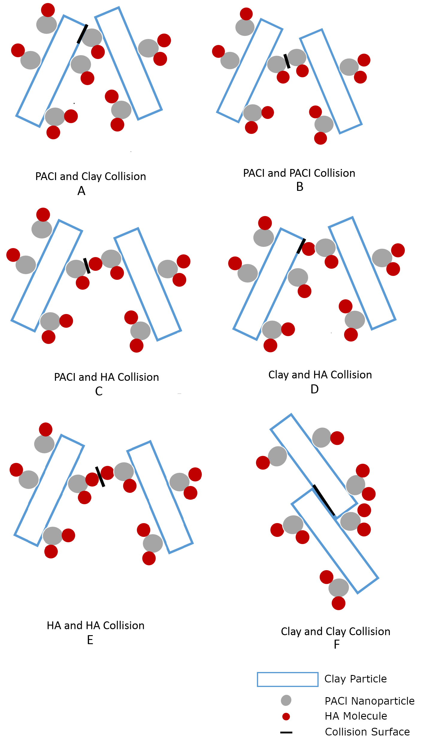
Fig. 124 Modes of collision between particles during flocculation.

Of these interactions considered in the model, the collisions that will result in attachment are assumed to involve at least one PACl nanoparticle surface (Fig. 124 A, B, C). The attachment efficiency is hypothesized to be the sum of probability of these three types of collisions, formally expressed as

\[\overline{\alpha }\ ={\overline{\alpha }}_\mathrm{PACl-Clay}+{\overline{\alpha }}_\mathrm{PACl-PACl}+{\overline{\alpha }}_\mathrm{HA-PACl},\]

where the subscripts define the two surfaces that are interacting. The overbars indicate that all of these represent mean probabilities for an entire suspension rather than the probabilities for specific particles.

The probability of a clay surface colliding with a PACl surface (Fig. 124 A) is equal to twice the probability that the first surface is clay (\(1-{\overline{\Gamma}}_\mathrm{PACl-Clay}\)) and the second surface is the PACl surface of a PACl-HA nanoaggregate (\(\left(1-{\overline{\Gamma}}_\mathrm{HA-PACl}\right){\overline{\Gamma}}_\mathrm{PACl-Clay}\)), since either of two colliding particles could provide the clay surface or the PACl surface,

\[{\overline{\alpha }}_\mathrm{PACl-Clay}=2\left(1-{\overline{\Gamma}}_\mathrm{PACl-Clay}\right)\left[\left(1-{\overline{\Gamma}}_\mathrm{HA-PACl}\right){\overline{\Gamma}}_\mathrm{PACl-Clay}\right].\]

The probability of a collision between the PACl surfaces of two PACl-HA nanoaggregates (\(\left(1-{\overline{\Gamma}}_\mathrm{HA-PACl}\right){\overline{\Gamma}}_\mathrm{PACl-Clay}\)) (Fig. 124 B) is given by

\[{\overline{\alpha}}_\mathrm{PACl-PACl}={\left[\left(1-{\overline{\Gamma}}_\mathrm{HA-PACl}\right){\overline{\Gamma}}_\mathrm{PACl-Clay}\right]}^2.\]

The probability of a collision between a PACl surface of a PACl-HA nanoaggregate (\(\left(1-{\overline{\Gamma}}_\mathrm{HA-PACl}\right){\overline{\Gamma}}_\mathrm{PACl-Clay}\)) and an HA surface of a PACl-HA nanoaggregate (\({\overline{\Gamma}}_\mathrm{HA-PACl}{\overline{\Gamma}}_\mathrm{PACl-Clay}\)) (Fig. 124 C), or vice versa, is given by

\[{\overline{\alpha }}_\mathrm{HA-PACl}=2\left[{\overline{\Gamma}}_\mathrm{PACl-Clay}\left(1-{\overline{\Gamma}}_\mathrm{HA-PACl}\right)\right]\left[{\overline{\Gamma}}_\mathrm{HA-PACl}{\overline{\Gamma}}_\mathrm{PACl-Clay}\right],\]

where the factor of 2 accounts for the possibility that either colliding particle could contribute either surface type.

The model accounting for the presence of humic acids is modified from the Pennock et al. (2018) model by redefining the attachment efficiency, \(\overline{\alpha }\), using Eq. 14 to account for the presence of humic acid.

The physical properties of humic acid vary with composition. The diameter of humic acid macromolecules is estimated to range from 4 nm to 110 nm ("{O}sterberg, 1993). Because of the variation in the size of humic acid macromolecules, the characteristic diameter of the humic acid macromolecules was used as a fitting parameter. Thus, there are two adjustable model parameters, \(k`(Equation :eq:`eq_AguaClara_Flocculation_Model\),), which accounts for the sedimentation capture velocity, and \(d_\mathrm{HA}\), which accounts for coagulant precipitate surface coverage by humic acid. These parameters were fit to results from observations taken with an influent turbidity of 50 NTU; the model was then validated by independently predicting results from experiments with an influent turbidity of 100 NTU.

Discussion

The solubility of humic acid is highly pH-dependent, and additional experimental results are needed to test the applicability of the model approach as a function of varying pH. The experimental conditions were designed to keep the pH relatively constant, and the pH change in the experiments was small (7.5 \(\pm\) 0.3).

The model considered flocculation in the presence of humic acid as a two-step process. Firstly, humic acid macromolecules attached to precipitated coagulant nanoparticles. Then, the partially-coated coagulant nanoaggregates could bind to clay and reactor wall surfaces. Humic acid and coagulant nanoparticles were treated as spheres when estimating the attachment efficiency based on surface coverage and probability. The diameter of precipitated PACl nanoparticles was experimentally measured to be 90 nm (Garland, 2017), and a humic acid macromolecule diameter of 75 nm best fit the observations. Wall loss of coagulant precipitates with humic acid nanoaggregates was considered while direct wall loss of humic acid macromolecules was not considered.

The characteristic humic acid dimension, \(d_\mathrm{HA}\), has a physical meaning, with the fitted value, 75 nm, falling within the range (4-110 nm) reported by "{O}sterberg (1993), and the model fits are well correlated to the observations. The predictive capability of the model was verified by predicting results under different experimental conditions with no additional adjustable parameters.

The flocculation model without the effects of humic acid shows that \(\mathrm{p}C^*\) is directly proportional to the log of the effective collision potential, \(\log(\overline{\alpha }\tilde{G}\theta {\phi }^{\frac{2}{3}})\), and this relationship is still present in the model with a modified attachment efficiency, \(\overline{\alpha },\) based on clay surface coverage by coagulant nanoparticles as adjusted for the presence of humic acids.

The form of the flocculation model equation sets the interactions between raw water properties (\({\phi }_0\)), influent particle surface area (which contributes to \({\overline{\Gamma}}_\mathrm{PACl-Clay}\)), coagulant precipitate size and dose (which contributes to \({\overline{\Gamma}}_\mathrm{PACl-Clay}\) and \({\overline{\Gamma}}_\mathrm{HA-PACl}\)) , humic acid molecule size and concentration (which contribute to \({\overline{\Gamma}}_\mathrm{HA-PACl}\)), flocculator design (\(\tilde{G}\theta\)), and clarifier design (\(k\)). In a gravity-powered water treatment plant operating at constant flow rate, the flocculator and clarifier parameters are constant. An increase in concentration of humic acid causes an increase in \({\overline{\Gamma}}_\mathrm{HA-PACl}\), which decreases \(\mathrm{p}C^*\) but can be compensated for by increasing coagulant dose.

The effect of the humic acid is to tie up a proportional amount of coagulant. The turbidity doesn’t begin to decrease until after all of the humic acid has coated the coagulant nanoparticles and thus it is finally possible for coagulant nanoparticles to remain sticky and attach to the inorganic particles (see Fig. 125 by Yingda Du, et al., 2019)

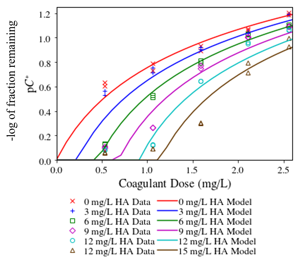
Fig. 125 Flocculation performance as a function of coagulant dose and humic acid concentration.

The data shown in Fig. 125 can also be plotted in a dimensionless form to show that all of the data converges reasonably well on a single model curve (see Fig. 126).

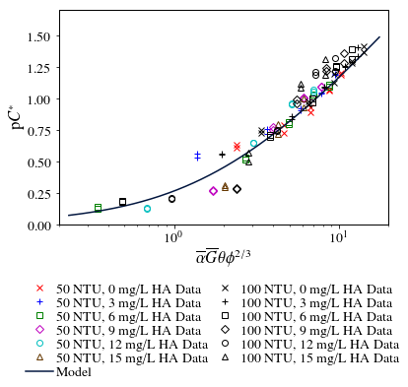
Fig. 126 Flocculation performance as a function of coagulant dose and humic acid concentration.

References

Amin, M., Safari, M., Maleki, A., Ghasemian, M., Rezaee, R., & Hashemi, H. (2012). Feasibility of humic substances removal by enhanced coagulation process in surface water. International Journal of Environmental Health Engineering. http://www.ijehe.org/text.asp?2012/1/1/29/99323

Benjamin, M. M., & Lawler, D. F. (2013). Water quality engineering: physical / chemical treatment processes. Hoboken, N.J.: Wiley.

BP-MWS, CIWS, & CUWS. (2016). Drinking Water Quality Report 2016. Ithaca, NY: Bolton Point Municipal Water System, City of Ithaca Water System, Cornell University Water System. Retrieved from https://fcs.cornell.edu/content/water-system-updates-and-water-quality-reports

Camp, T. R. (1953). Flocculation and Flocculation Basins. American Society of Civil Engineers.

Chow, C. W. K., Fabris, R., Leeuwen, J. van, Wang, D., & Drikas, M. (2008). Assessing Natural Organic Matter Treatability Using High Performance Size Exclusion Chromatography. Environmental Science & Technology, 42(17), 6683–6689. https://doi.org/10.1021/es800794r

Cleasby, J. (1984). Is Velocity Gradient a Valid Turbulent Flocculation Parameter? Journal of Environmental Engineering, 110(5), 875–897. https://doi-org.proxy.library.cornell.edu/10.1061/(ASCE)0733-9372(1984)110:5(875)

Davis, J. A. (1982). Adsorption of natural dissolved organic matter at the oxide/water interface. Geochimica et Cosmochimica Acta, 46(11), 2381–2393. https://doi.org/10.1016/0016-7037(82)90209-5

Fosso-Kankeu, E., Webster, A., Ntwampe, I. O., & Waanders, F. B. (2017). Coagulation/Flocculation Potential of Polyaluminium Chloride and Bentonite Clay Tested in the Removal of Methyl Red and Crystal Violet. Arabian Journal for Science and Engineering, 42(4), 1389–1397. https://doi.org/10.1007/s13369-016-2244-x

Garland, C. A. (2017). Uncovering the Mysteries of the Floc Blanket: An Exploration with Inlet Jets, Flocculators, and Polyaluminum Chloride Precipitates (Ph.D. thesis). Cornell University, United States – New York. Retrieved from https://search.proquest.com/docview/1959337645/abstract/A3C1677072644AD5PQ/1

Granger, R. A. (1995). Fluid Mechanics. New York: Dover Publications.

Hu, C., Liu, H., Qu, J., Wang, D., & Ru, J. (2006). Coagulation Behavior of Aluminum Salts in Eutrophic Water: Significance of Al13 Species and pH Control. Environmental Science & Technology, 40(1), 325–331. https://doi.org/10.1021/es051423+

Hua, G., & Reckhow, D. A. (2008). Relationship between Brominated THMs, HAAs, and Total Organic Bromine during Drinking Water Chlorination. In T. Karanfil, S. W. Krasner, P. Westerhoff, & Y. Xie (Eds.), Disinfection By-Products in Drinking Water (Vol. 995, pp. 109–123). Washington, DC: American Chemical Society. https://doi.org/10.1021/bk-2008-0995.ch008

Integrated design of water treatment facilities: Susumu Kawamura. John Wiley & Sons, Inc.: New York, NY 1991. (pp. 658, ISBN 0-471-61591-9) $69.95 hardcover. (1992). Waste Management, 12(1), 101. https://doi.org/10.1016/0956-053X(92)90024-D

Ives, K. J. (1968). Theory of operation of sludge blanket clarifiers. Proceedings of the Institution of Civil Engineers, 39(2), 243–260. https://doi.org/10.1680/iicep.1968.8090

Jarvis, P., Jefferson, B., Gregory, J., & Parsons, S. A. (2005). A review of floc strength and breakage. Water Research, 39(14), 3121–3137. https://doi.org/10.1016/j.watres.2005.05.022

Kundu, P. K., & Cohen, I. M. (2008). Fluid mechanics. Amsterdam; Boston: Academic Press.

Letterman, R. D. (1999). Water quality and treatment: a handbook of community water supplies (5th ed.). New York: McGraw-Hill.

Li, W., Liao, P., Oldham, T., Jiang, Y., Pan, C., Yuan, S., & Fortner, J. D. (2018). Real-time evaluation of natural organic matter deposition processes onto model environmental surfaces. Water Research, 129, 231–239. https://doi.org/10.1016/j.watres.2017.11.024

Lin, J.-L., Huang, C., Dempsey, B., & Hu, J.-Y. (2014). Fate of hydrolyzed Al species in humic acid coagulation. Water Research, 56, 314–324. https://doi.org/10.1016/j.watres.2014.03.004

Matilainen, A., Vepsäläinen, M., & Sillanpää, M. (2010). Natural organic matter removal by coagulation during drinking water treatment: A review. Advances in Colloid and Interface Science, 159(2), 189–197. https://doi.org/10.1016/j.cis.2010.06.007

Marhaba, T. F., Pu, Y., & Bengraine, K. (2003). Modified dissolved organic matter fractionation technique for natural water. Journal of Hazardous Materials, 101(1), 43–53. https://doi.org/10.1016/S0304-3894(03)00133-X

O’Melia, C. R. (1972). Coagulation and flocculation. In W. J. Weber (Ed.), Physicochemical processes for water quality control. New York: Wiley-Interscience.

Österberg, R., Lindovist, I., & Mortensen, K. (1993). Particle Size of Humic Acid. Soil Science Society of America Journal, 57(1), 283–285. https://www.nbi.dk/~kell/publ/1993_SoilSciSocAJ_HumicAcid.pdf

Pennock, William H., Weber-Shirk, Monroe, & Lion, Leonard W. (2018). A Hydrodynamic and Surface Coverage Model Capable of Predicting Settled Effluent Turbidity Subsequent to Hydraulic Flocculation. Environmental Engineering Science, 35(12). https://doi.org/10.1089/ees.2017.0332

Schulz, C. R., & Okun, D. A. (1984). Surface water treatment for communities in developing countries. New York: Wiley.

Sharp, E. L., Jarvis, P., Parsons, S. A., & Jefferson, B. (2006). Impact of fractional character on the coagulation of NOM. Colloids and Surfaces A: Physicochemical and Engineering Aspects, 286(1–3), 104–111. https://doi.org/10.1016/j.colsurfa.2006.03.009

Sigma-Aldrich. (2014). Humic acid sodium salt (H16752) (Safety Data Sheet) (p. 7). St. Louis, MO.

Soh, Y. C., Roddick, F., & Leeuwen, J. van. (2008). The impact of alum coagulation on the character, biodegradability and disinfection by-product formation potential of reservoir natural organic matter (NOM) fractions. Water Science and Technology; London, 58(6), 1173–1179. http://dx.doi.org/10.2166/wst.2008.475

Swetland, K. A., Weber-Shirk, M. L., & Lion, L. W. (2013). Influence of Polymeric Aluminum Oxyhydroxide Precipitate-Aggregation on Flocculation Performance. Environmental Engineering Science, 30(9), 536–545. https://doi.org/10.1089/ees.2012.0199

Swetland, K. A., Weber-Shirk, M. L., & Lion, L. W. (2014). Flocculation-Clarification Performance Model for Laminar-Flow Hydraulic Flocculation with Polyaluminum Chloride and Aluminum Sulfate Coagulants. Journal of Environmental Engineering, 140(3), 04014002. https://doi.org/10.1061/(ASCE)EE.1943-7870.0000814

Tse, I. C., Swetland, K., Weber-Shirk, M. L., & Lion, L. W. (2011). Method for quantitative analysis of flocculation performance. Water Research, 45(10), 3075–3084. https://doi.org/10.1016/j.watres.2011.03.021

Van Benschoten, J. E., & Edzwald, J. K. (1990). Chemical aspects of coagulation using aluminum salts—I. Hydrolytic reactions of alum and polyaluminum chloride. Water Research, 24(12), 1519–1526. https://doi.org/10.1016/0043-1354(90)90086-L

Weber-Shirk, M. L. (2016). ProCoDA: An Automated Method for Testing Process Parameters. Retrieved October 30, 2015, from https://confluence.cornell.edu/display/AGUACLARA/ProCoDA

Weber-Shirk, M. L., & Lion, L. W. (2010). Flocculation model and collision potential for reactors with flows characterized by high Peclet numbers. Water Research, 44(18), 5180–5187. https://doi.org/10.1016/j.watres.2010.06.026

Willis, R. M. (1978). Tubular Settlers—A Technical Review. Journal (American Water Works Association), 70(6), 331–335.

Xiong, X., Wu, X., Zhang, B., Xu, H., & Wang, D. (2018). The interaction between effluent organic matter fractions and Al2(SO4)3 identified by fluorescence parallel factor analysis and FT-IR spectroscopy. Colloids and Surfaces A: Physicochemical and Engineering Aspects, 555, 418–428. https://doi.org/10.1016/j.colsurfa.2018.07.026

Yan, M., Wang, D., Ni, J., Qu, J., Chow, C. W. K., & Liu, H. (2008). Mechanism of natural organic matter removal by polyaluminum chloride: Effect of coagulant particle size and hydrolysis kinetics. Water Research, 42(13), 3361–3370. https://doi.org/10.1016/j.watres.2008.04.017

[BL13]

Mark M. Benjamin and Desmond F. Lawler. Water quality engineering: physical / chemical treatment processes. Wiley, Hoboken, N.J., July 2013. ISBN 978-1-118-16965-0. URL: http://encompass.library.cornell.edu/cgi-bin/checkIP.cgi?access=gateway_standard%26url=http://search.ebscohost.com/login.aspx?direct=true&scope=site&db=nlebk&db=nlabk&AN=631668 (visited on 2017-02-22).

[BB98]

Markus Boller and Stefan Blaser. Particles under stress. Water Science and Technology, 37(10):9–29, May 1998. URL: http://wst.iwaponline.com/content/37/10/9 (visited on 2016-08-21).

[DC08]

Mackenzie Leo Davis and David A Cornwell. Introduction to Environmental Engineering. McGraw-Hill Companies, Dubuque, IA, 4th edition, 2008. ISBN 978-0-07-242411-9 978-0-07-125922-4 978-7-302-15210-1. OCLC: 70708094.

[GWSL16]

Casey Garland, Monroe Weber-Shirk, and Leonard W. Lion. Revisiting Hydraulic Flocculator Design for Use in Water Treatment Systems with Fluidized Floc Beds. Environmental Engineering Science, 34(2):122–129, August 2016. URL: http://online.liebertpub.com/doi/abs/10.1089/ees.2016.0174 (visited on 2017-02-22), doi:10.1089/ees.2016.0174.

[Gra95] (1,2)

Robert Alan Granger. Fluid Mechanics. Dover Publications, New York, 1995. ISBN 978-1-62198-654-6 1-62198-654-3.

[ML00]

G. L. McConnachie and J. Liu. Design of baffled hydraulic channels for turbulence-induced flocculation. Water Research, 34(6):1886–1896, April 2000. URL: https://www.sciencedirect.com/science/article/pii/S0043135499003292 (visited on 2016-04-08), doi:10.1016/S0043-1354(99)00329-2.

[MCM+12]

Jasmin Mertens, Barbara Casentini, Armand Masion, Rosemarie Pöthig, Bernhard Wehrli, and Gerhard Furrer. Polyaluminum chloride with high Al30 content as removal agent for arsenic-contaminated well water. Water Research, 46(1):53–62, January 2012. URL: https://www.sciencedirect.com/science/article/pii/S0043135411006294 (visited on 2017-03-31), doi:10.1016/j.watres.2011.10.031.

[PCWSL16] (1,2,3,4,5,6)

William H. Pennock, Felice C. Chan, Monroe L. Weber-Shirk, and Leonard W. Lion. Theoretical Foundation and Test Apparatus for an Agent-Based Flocculation Model. Environmental Engineering Science, July 2016. URL: http://online.liebertpub.com/doi/abs/10.1089/ees.2015.0558 (visited on 2016-07-07), doi:10.1089/ees.2015.0558.

[SWSL15]

Siwei Sun, Monroe Weber-Shirk, and Leonard W. Lion. Characterization of Flocs and Floc Size Distributions Using Image Analysis. Environmental Engineering Science, 33(1):25–34, November 2015. URL: http://online.liebertpub.com/doi/10.1089/ees.2015.0311 (visited on 2016-05-17), doi:10.1089/ees.2015.0311.

[SWSL13]

Karen A. Swetland, Monroe L. Weber-Shirk, and Leonard W. Lion. Influence of Polymeric Aluminum Oxyhydroxide Precipitate-Aggregation on Flocculation Performance. Environmental Engineering Science, 30(9):536–545, September 2013. URL: http://online.liebertpub.com/doi/abs/10.1089/ees.2012.0199 (visited on 2017-06-09), doi:10.1089/ees.2012.0199.

[SWSL14] (1,2,3,4,5,6)

Karen A. Swetland, Monroe L. Weber-Shirk, and Leonard W. Lion. Flocculation-Clarification Performance Model for Laminar-Flow Hydraulic Flocculation with Polyaluminum Chloride and Aluminum Sulfate Coagulants. Journal of Environmental Engineering, 140(3):04014002, March 2014. URL: http://ascelibrary.org/doi/10.1061/%28ASCE%29EE.1943-7870.0000814 (visited on 2015-06-26), doi:10.1061/(ASCE)EE.1943-7870.0000814.

[WZL+15] (1,2,3)

Ning Wei, Zhongguo Zhang, Dan Liu, Yue Wu, Jun Wang, and Qunhui Wang. Coagulation behavior of polyaluminum chloride: Effects of pH and coagulant dosage. Chinese Journal of Chemical Engineering, 23(6):1041–1046, June 2015. URL: https://www.sciencedirect.com/science/article/pii/S1004954115000804 (visited on 2015-10-03), doi:10.1016/j.cjche.2015.02.003.

[BPMWSCIWSCUWS16]

BP-MWS, CIWS, and CUWS. Drinking Water Quality Report 2016. Technical Report, Bolton Point Municipal Water System, City of Ithaca Water System, Cornell University Water System, Ithaca, NY, 2016. URL: https://energyandsustainability.fs.cornell.edu/file/AWQR_2016%20final.pdf.